 Products Home / Drivers & Mounts / OEM Laser Diode & TEC Systems / IC Temperature Controllers in SMT or THT Packages
IC Temperature Controllers in SMT or THT Packages
- Compact, Highly Integrated TEC Drivers
- Deliver Current up to ±1.5 A or ±2.0 A to TEC
- Designed for OEM, Custom, and Embedded Systems
- Volume Pricing Available
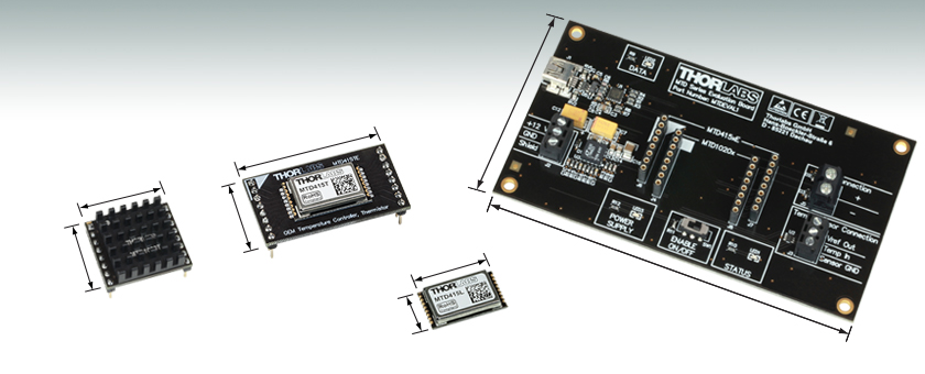
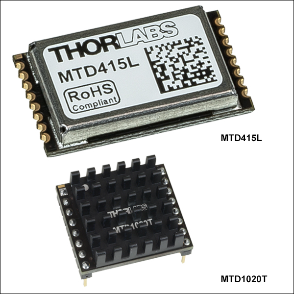
MTD415L
SMT Package for ±1.5 A and
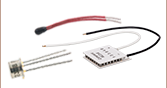
LMT84 IC Temperature Sensor
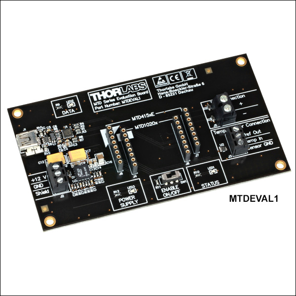
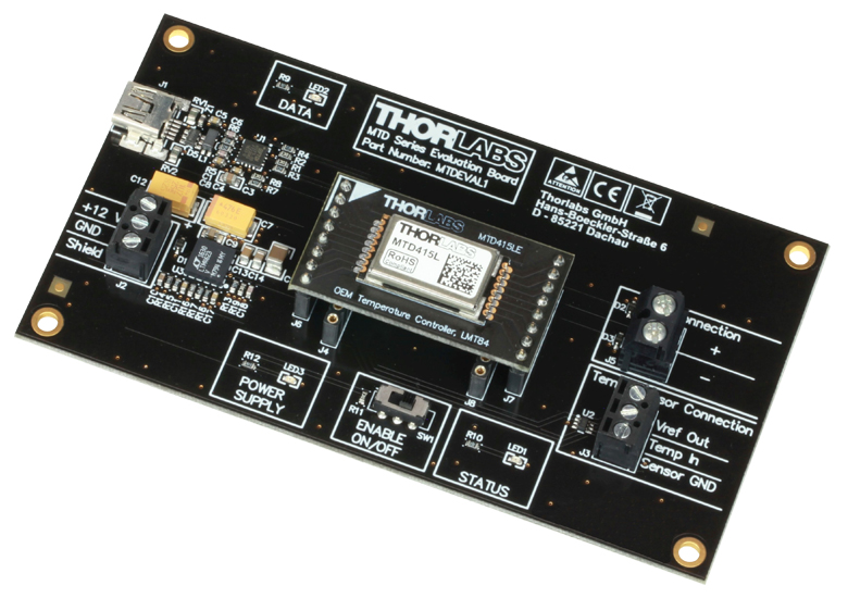
MTDEVAL1
Evaluation Board for OEM TEC Drivers
21.0 mm
12.4 mm
39.6 mm
21.5 mm
MTD1020T
THT Package for ±2.0 A and 10 kΩ Thermistor
114.5 mm
64.0 mm
MTD415TE
Adapter PCB with Mounted MTD415T
SMT Package
27.0 mm
21.0 mm


Please Wait
| Table 1.1 Key Featuresa | |||
|---|---|---|---|
| Item # | MTD415L(E) | MTD415T(E) | MTD1020T |
| Supported Temperature Sensor | LMT84 IC | 10 kΩ Thermistor | |
| Output Current (See Graphs on Specs Tab) | Up to ±1.5 A | Up to ±2.0 A | |
| TEC Compliance Voltage | 4.0 V | 10.0 V | |
| Maximum Output Power (See Graphs on Specs Tab) |
Up to 6.0 W | Up to 20.0 W | |
| Noise and Ripple (Typical) | 150 mA (Peak-Peak) or 87 mA RMS | ||
| Temperature Stability (Typical) | 100 mK | ||
| Data Sheet (Click for PDF) | |||
Volume Pricing & OEM Support
Thorlabs' production facilities are capable of manufacturing TEC controllers in high volumes, and we pass the savings associated with planned production on to our customers.
Contact our OEM team to learn more. An OEM specialist will contact you within 24 hours or on the next business day.

Click to Enlarge
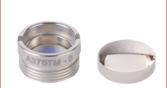
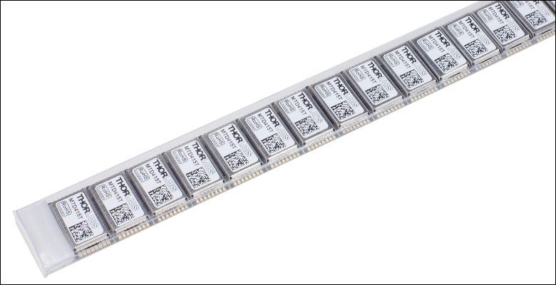
Upon request, large-quantities of MTD415 series drivers in SMT packages can be delivered in an IC tube.
Click to Enlarge
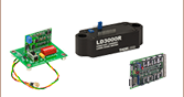
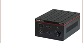
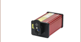
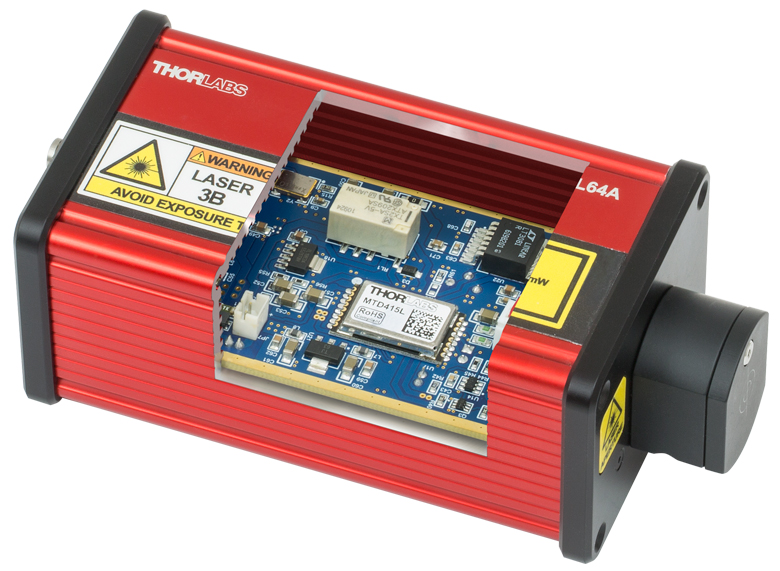
Figure 1.2 Application Example:
MTD415L TEC drivers are used for temperature regulation in Thorlabs' Nanosecond Pulsed Laser Systems, as shown in this cutaway view of the NPL64A.
Features
- Integrated Drivers with Digital PID Loops for TECs
- Three Packages Available: THT, SMT, and SMT on Daughterboard
- Low Output Current Noise: ≤150 mA
- Units can be Controlled via a PC
- Accepts Serial Commands over UART Entered through a Command Line Interface
- GUI to Adjust Settings and Monitor Driver Performance (See Software Tab)
- Evaluation Board Available for Testing and Evaluating Driver Settings
Applications
- Ideal for Small Assemblies that Use Thermoelectric Coolers
- Active Cooling and Temperature Stabilization for
- Laser Modules and Laser Diodes
- WDM and DWDM Laser Diodes
- EDFA Optical Amplifiers
- Photodetectors and Photodiodes
- Automated Test Equipment (ATE)
Thorlabs offers several complete driver module options designed for OEM system integration. The high compliance voltage of the MTD1020T, which is offered in a through-hole technology (THT) package, allows it to deliver the maximum ±2.0 A TEC current into load resistances up to 5 Ω. The MTD415 Series, which are offered in surface-mount technology (SMT) packages and as SMT packages mounted on daughterboards, deliver TEC current up to ±1.5 A depending on the load resistance. Please see the Specs tab for typical performance plots and specifications.
Each of these OEM-grade TEC drivers employs a digital control loop to regulate the current output. These PID control loops enable our TEC drivers to provide faster temperature settling times and better stability than drivers using PI control loops. True bipolar operation allows the output current to reach 0 A without "dead zones" or other nonlinearities at low TEC currents. The complete on-chip power stage and thermal control loop circuitry minimize external components while maintaining high efficiency and low output current noise of ≤150 mA. The output current is directly controlled to eliminate current surges to the TEC, while an adjustable TEC current limit provides protection against overdriving the cooler.
Computer Control
These drivers use a UART digital control interface that allows quick access to PID settings, all other system parameters, and digital measurement data, enabling easy integration into a variety of systems. The TEC drivers are controlled via a PC using either the programming commands outlined in the TEC driver data sheets (linked to in Table 1.1) or a GUI for Windows® operating systems (see the Software tab). This GUI provides a simple means of optimizing the TEC driver settings to a specific thermal load, as well as graphical output that tracks the TEC performance. See the PID Oscillation Test tab for an example of how to set the PID parameters using the GUI.
Evaluation Board
For those customers interested in evaluating the performance of the MTD series TEC drivers and optimizing their response to a particular thermal load, we offer the MTDEVAL1 evaluation board. The evaluation board has a built-in UART-to-USB adapter that allows commands sent from a PC to address the mounted driver.
All technical data are valid at 23 ± 5 °C and 45 ± 15% relative humidity (non-condensing).
| Table 2.1 TEC Driver Specifications | |||
|---|---|---|---|
| Item # | MTD415L(E) | MTD415T(E) | MTD1020T |
| TEC Current Output | |||
| Maximum Output Current | Up to ±1.5 A (See Figures 2.4, 2.5, 2.6, and 2.7) |
Up to ±2.0 A 2.6, and 2.7) |
|
| TEC Compliance Voltage | 4.0 V | 10.0 V | |
| Maximum Output Power | Up to 6.0 W | Up to 20.0 W | |
| Measurement Resolution | 3 mA (Typical) 8 mA (Max) |
5 mA (Typical) 10 mA (Max) |
|
| Measurement Accuracy | ±50 mA | ||
| Noise and Ripple (Typical) | 150 mA (Peak-Peak) or 87 mA RMS | ||
| TEC Current Limit | |||
| Setting Rangea | 0 to 1.5 A | 0 to 2.0 A | |
| Setting Resolution | 1 mA | ||
| Setting Accuracy | ±50 mA | ||
| Temperature Sensor | |||
| Supported Sensor | LMT84 IC Sensor or Similar |
10 kΩ Thermistorb | |
| Maximum Temperature Control Rangec |
+5 °C to +45 °C | ||
| Temperature Setting Resolution | 1 mK | ||
| Temperature Measurement Resolutiond | 2 mK (Typical) 10 mK (Max) |
3 mK (Typical) 10 mK (Max) |
|
| Absolute Temperature Accuracyc | ±0.5 °C | ||
| Temperature Stability (Typical)e | 100 mK | ||
| Temperature Coefficient | <20 mK/°C | ||
| Recommended Operating Conditions | |||
| Supply Input Voltage | 4.5 V to 5.5 V | 11.5 V to 12.5 Vf | |
| -20 °C to 60 °C | |||
| 10 Minutes | |||
| Programming Interface | |||
| Type | UART | ||
| Voltage Level | 3.3 V Logic Level; Input 5 V Tolerant | ||
| Data Rate | 115,200 bps; 8 Data Bits, 1 Stop Bit | ||
| Safety Features | |||
| Safety Features | TEC Current Limit Sensor Fault Protection TEC Open Circuit Protection Temperature Setpoint Limit Temperature Window Protection Delay Over Temperature Protection |
||
| Environmental | |||
| Storage Temperature | -40 °C to 100 °C | ||
| Table 2.2 TEC Driver Absolute Maximum Ratings | ||||
|---|---|---|---|---|
| Item # | MTD415L(E) | MTD415T(E) | MTD1020T | |
| Supply Input Voltage | 4.5 V to 6 V | 11.5 V to 13.0 V | ||
| Supply Input Current | 1.6 A | 2.3 A | ||
| TEC Output Current | -1.5 A to +1.5 A | -2.0 A to +2.0 A | ||
| 4.0 V | 10.0 V | |||
| 6.0 W | 20.0 W | |||
| Power Dissipation | 1.5 W | 4.0 W | ||
(With Respect to Ground Terminal) |
VDD | -0.3 V to +6 V | -0.3 V to +13.0 V | |
| TX | - | -0.3 V to +3.6 V | ||
| ENABLE, RX | -0.3 V to (VDD + 0.3 V) | |||
| TEC-, TEC+ | 0.0 V to +13.0 V | |||
| TEMP | -0.3 V to +3.3 V | |||
| Maximum Output Current (STATUS, TX) | 10 mA | |||
| Maximum Input Current (ENABLE, RX) | 10 mA | |||
| Ambient Operating Temperatures | -40 °C to 70 °C | |||
| Table 2.3 TEC Controller Package Dimensions | |||
|---|---|---|---|
| Item # | Package Type | Dimensions | Approximate Weight |
| MTD415L | SMTa | (0.83" x 0.49" 0.12") |
2 g |
| MTD415LE | Daughterboard | (1.56" x 0.85" x 0.55" ) |
4 g |
| MTD415T | SMTa | (0.83" x 0.49" 0.12") |
2 g |
| MTD415TE |
Daughterboard | (1.56" x 0.85" x 0.55" ) |
4 g |
| MTD1020T | THTb | (1.06" x 0.83" x 0.41") |
8 g |
MTD415 Series Typical Output Characteristics
Click to Enlarge
Figure 2.4 MTD415 Series deliver the maximum output power of 6 W into a load resistance of 2.66 Ω when operating under recommended conditions. The shaded range corresponds to load resistances less than 2.66 Ω, for which the maximum output power depends on environmental conditions.
Click to Enlarge
Figure 2.5 MTD415 Series deliver the maximum TEC current of 1.5 A into a load resistance of 2.66 Ω when operating under recommended conditions. The maximum output current drops for higher load resistances due to the limit of the compliance voltage. The shaded range corresponds to load resistances less than 2.66 Ω, for which the maximum output current depends on environmental conditions.
MTD1020T Typical Output Characteristics
Click to Enlarge
Figure 2.6 MTD1020T delivers the maximum output power of 20 W into a load resistance of 5 Ω, when operating under recommended conditions and actively cooled, or for ambient temperatures between -20 °C and 20 °C when convection cooled. The red curve applies to an ambient temperature of 60 °C and convection cooling.
Click to Enlarge
Figure 2.7 MTD1020T delivers the maximum TEC current of 2.0 A into load resistances up to 5 Ω, when operating under recommended conditions and actively cooled with 2 m/s forced air or cooling methods at least equally effective. When convection cooled, the maximum 2.0 A current can be delivered into any load resistances up to 5 Ω for ambient temperatures up to 20 °C. Other cooling methods may give intermediate results.
MTDEVAL1 Evaluation Board
| Table 2.8 Specifications | |
|---|---|
| Supply Input Voltage | 11.5 VDC to 13.0 VDC |
| Supply Input Current (Maximum) | 2.3 A |
| USB Connection | USB Mini B |
| Operating Temperature Range | 0 °C to 40 °C |
| Storage Temperature Range | -40 °C to 70 °C |
| Dimensions | (4.51" x 2.52" x 0.66") |
| Weight | 40 g |
Click on the following links to move to the different sections in this discussion.
- Pin Layout of the MTD415 Series
- Typical Application Circuits for the MTD415 Series
- Pin Layout of the MTD1020T
- Typical Application Circuit for the MTD1020T
Pin Layout of the MTD415 Series
These pin assignments correspond to viewing the driver from the top when the engraving on the driver is right-side up.
Land Pattern Data of the MTD415L(E) and MTD415T(E)
| MTD415L(E) TEC Driver | ||
|---|---|---|
| Pin | Name | Description |
| 1 | VDD | Supply Voltage Input (+4.5 V to +5.5 V) |
| 2 | GND | Supply Voltage Ground |
| 3 | GND | Supply Voltage Ground |
| 4 | DNC | Do Not Connect |
| 5 | DNC | Do Not Connect |
| 6 | VREF | Reference Output Voltage for LMT84 Temperature Sensor (1.8 V) |
| 7 | TEMP | LMT84 Temperature Sensor Input |
| 8 | GNDS | Temperature Sensor Ground This ground connection should be wired separately and not be shared with other Ground pins. |
| 9 | GND | Supply Voltage Ground |
| 10 | ENABLE | Enable Signal Input (Low-Active) Low = Enabled, High = Disabled Can be Connected Directly to GND |
| 11 | STATUS | Status Signal Output (Can be Left Floating) High = Temperature within Defined Temperature Window Low = Temperature outside Programmed Temperature Window or an Error Occurred |
| 12 | TX | Digital Interface Transmit Signal |
| 13 | RX | Digital Interface Receive Signal |
| 14 | GND | Supply Voltage Ground |
| 15 | TEC - | TEC Element Negative Connection (Connect to Positive Terminal on TEC) |
| 16 | TEC + | TEC Element Positive Connection (Connect to Negative Terminal on TEC) |
| MTD415T(E) TEC Driver | ||
|---|---|---|
| Pin | Name | Description |
| 1 | VDD | Supply Voltage Input (+4.5 V to +5.5 V) |
| 2 | GND | Supply Voltage Ground |
| 3 | GND | Supply Voltage Ground |
| 4 | DNC | Do Not Connect |
| 5 | DNC | Do Not Connect |
| 6 | VREF | Reference Output Voltage for Thermistor Temperature Sensor (1.8 V) |
| 7 | TEMP | Thermistor Temperature Sensor Input |
| 8 | GNDS | Temperature Sensor Ground Can be used for Shielding Purposes or Left Open |
| 9 | GND | Supply Voltage Ground |
| 10 | ENABLE | Enable Signal Input (Low-Active) Low = Enabled, High = Disabled Can be Connected Directly to GND |
| 11 | STATUS | Status Signal Output (Can be Left Floating) High = Temperature within Defined Temperature Window, Low = Temperature Outside Programmed Temperature Window or an Error Occurred |
| 12 | TX | Digital Interface Transmit Signal |
| 13 | RX | Digital Interface Receive Signal |
| 14 | GND | Supply Voltage Ground |
| 15 | TEC - | TEC Element Negative Connection (Connect to Positive Terminal on TEC) |
| 16 | TEC + | TEC Element Positive Connection (Connect to Negative Terminal on TEC) |
Typical Application Circuits for the MTD415 Series
Click to Enlarge
Sample External Circuit for MTD415L TEC Driver
Click to Enlarge
Sample External Circuit for MTD415T TEC Driver
Pin Layout of the MTD1020T
These pin assignments correspond to viewing the driver from the top when the engraving on the driver is right-side up.
Top View of the MTD1020T
| MTD1020T TEC Driver | ||
|---|---|---|
| Pin | Name | Description |
| 1 | VDD | Supply Voltage Input (+11.5 V to +12.5 V) |
| 2 | GND | Supply Voltage Ground |
| 3 | GND | Supply Voltage Ground |
| 4 | DNC | Do Not Connect |
| 5 | DNC | Do Not Connect |
| 6 | VREF | Reference Output Voltage for Thermistor Temperature Sensor (1.24 V) |
| 7 | TEMP | Thermistor Temperature Sensor Input |
| 8 | GNDS | Temperature Sensor Ground Can be used for Shielding Purposes or Left Open |
| 9 | GND | Supply Voltage Ground |
| 10 | ENABLE | Enable Signal Input (Low-Active) Low = Enabled, High = Disabled Can be Connected Directly to GND |
| 11 | STATUS | Status Signal Output (Can be Left Floating) High = Temperature within Defined Temperature Window, Low = Temperature Outside Programmed Temperature Window or an Error Occurred |
| 12 | TX | Digital Interface Transmit Signal |
| 13 | RX | Digital Interface Receive Signal |
| 14 | TEC - | TEC Element Negative Connection |
| 15 | TEC + | TEC Element Positive Connection |
| 16 | GND | Supply Voltage Ground |
Click to Enlarge
Sample External Circuit for MTD1020T TEC Driver
Click to Enlarge
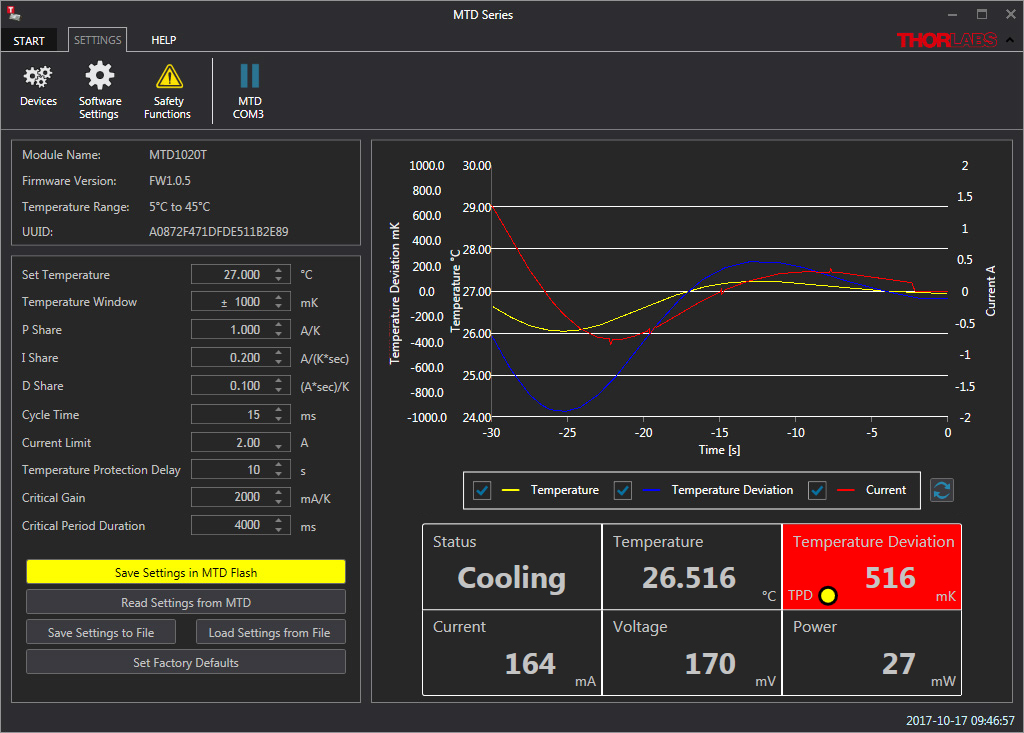
Figure 4.1 The OEM Temperature Controller GUI Interface
GUI and Drivers for OEM Temperature Controllers and Evaluation Board
The download button provides a link to the GUI and drivers that allow these TEC drivers to be controlled via a PC with a Windows® operating system. The software can be used to perform an oscillation test and can automatically calculate the optimal P, I, and D parameters for a setup using the results. For details on the oscillation test procedure and an introduction to PID circuits, see the PID Oscillation Test tab.
Software
Version 1.5 (April 21, 2021)
This is a software package with a GUI and drivers for Thorlabs' OEM TEC drivers in SMT packages.
| Table 5.2 Oscillation Test Starting Parameters | |
|---|---|
| Set Temperature | 25.000 °C |
| P Share | 1000 mA/K |
| I Share | 0 A/Ks |
| D Share | 0 As/K |
| Cycle Time | 30 ms |
Click to Enlarge
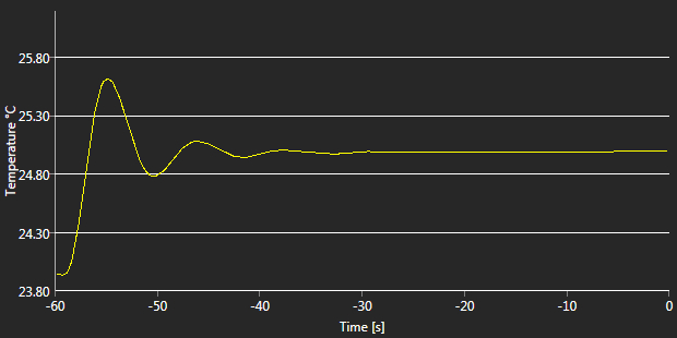
Figure 5.3 Initial Settling Behavior after TEC is Enabled
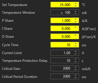
Figure 5.1 Starting Parameters for the Oscillation Test
Oscillation Test to Set PID Parameters
Each MTD415 and MTD1020T module incorporates a digital PID controller. The P, I, and D shares can be programmed manually or calculated automatically by the firmware by entering the results of a loop oscillation test. This test can be performed using the GUI available on the Software tab, and provides a convenient method for optimizing the PID parameters.
Before running the test, the following preconditions must be met:
- TEC Current Limit is Set to 1 A
- All Connections are Made Properly
- Temperature Window Settings in the GUI's Software Settings
- Set the Temperature Window to ±100 mK
- Display only the Actual Temperature
- Set the X-Axis of the Temperature Graph to a Max Time of 60 s
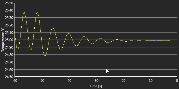
First, enter the PID loop settings shown in Table 5.2. These initial settings allow the user to observe the temperature settling process, as typically no oscillations will appear when the driver is operated with these settings. Then, enable the TEC. The actual temperature, measured by the unit and recorded on the graph in the GUI, will approximate the set value.

Click to Enlarge
Figure 5.5 P Share = 5000 mA/K
Click to Enlarge
Figure 5.4 P Share = 10,000 mA/K
Click to Enlarge
Figure 5.7 P Share = 2000 mA/K
Click to Enlarge
Figure 5.6 P Share = 3000 mA/K
Click to Enlarge
Figure 5.9 P Share = 2800 mA/K

Click to Enlarge
Figure 5.8 P Share = 2600 mA/K
Click to Enlarge
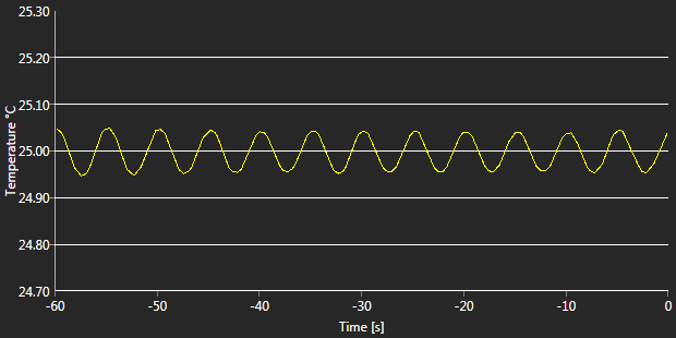
Figure 5.11 P Share = 2650 mA/K

Click to Enlarge
Figure 5.10 P Share = 2700 mA/K
The critical P share (critical gain) is the value at which the system starts to oscillate for a minimum of 20 cycles without a drop in amplitude as a reaction to a change in the temperature setpoint. The procedure for the oscillation loop test used to find the critical P share is described as follows: with I and D set at zero, the P share value is set high enough that the loop oscillates without damping. Then, smaller P share values are tested until the oscillations are damped. The P share is increased again by a smaller amount until the loop begins to oscillate continuously again, and then decreased to find the threshold where the oscillations become damped again. After each change in the P share value, the temperature setpoint must be changed slightly to trigger the loop with the new P share setting. The process is repeated until the minimum P share value for the loop to oscillate without damping is found; this is the critical P share value.
The following example illustrates how the oscillation loop test procedure is carried out. For this case, a passive thermal load consisting of a 60 mm x 60 mm x 25 mm radiator was connected to a TEC and a temperature sensor.
- After entering the initial settings and enabling the TEC (Figure 5.1), the temperature begins to settle (Figure 5.3).
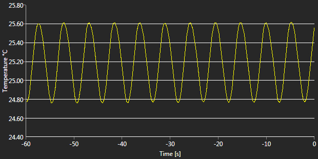
- The P share is set to 10,000 mA/K, since this value is high enough that it will trigger the loop to oscillate for almost any thermal load. Then, the set temperature is increased by 0.1 K to 25.1 °C. The loop begins to show strong oscillations (Figure 5.4).
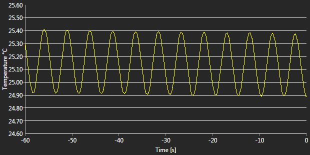
- The P share is lowered to 5000 mA/K and the set temperature is decreased to 25.0 °C again. The loop continues to oscillate (Figure 5.5).
- The P share is lowered again to 3000 mA/K and the set temperature increased to 25.1 °C. The loop continues to oscillate (Figure 5.6).
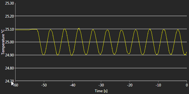
- The P share is lowered to 2000 mA/K and the set temperature is decreased to 25.0 °C. The oscillations are now damped (Figure 5.7).
- The P share is increased to 2600 mA/K and the set temperature to 25.1 °C. The oscillations are still damped (Figure 5.8).
- The P share is increased again to 2800 mA/K and the set temperature decreased to 25.0 °C. The loop begins to oscillate again (Figure 5.9).
- The P share is lowered to 2700 mA/K and the set temperature increased to 25.1 °C. The loop continues to oscillate (Figure 5.10).
- The P share is lowered to 2650 mA/K and the set temperature decreased to 25.0 °C. The loop still oscillates (Figure 5.11).
- At this point, we know that at 2600 mA/K, the oscillations were damped (step 6), so 2650 mA/K is the lowest P share value for which the loop will oscillate continuously. This value will be used for the critical gain.
- Use the diagram from step 9 (Figure 5.11) to calculate the critical period (i.e., the time of one oscillation). Count the number of oscillations across the 60 s observation window and divide 60 by this number. In this case, there are 11.8 periods, so each period has a duration of approximately 5.085 s.
- Enter the critical gain (step 10) and critical period duration (step 11) into the GUI (Figure 5.12). Press enter to trigger the calculation of the PID shared and cycle time by the firmware. The calculated loop parameters will be displayed immediately (Figure 5.13).
Typically, the PID optimization for settling behavior is finished at this point. If required, the PID values and the cycle time can be manually fine-tuned in order to optimize the loop response to changes of the thermal load.
Saving the PID Parameters for Later Use
These TEC drivers are designed with a temporary volatile memory and a non-volatile flash memory. As the flash memory has a limited number of erase-write cycles, parameters entered into the GUI will be saved in the volatile memory only, unless otherwise directed by the user. This means that these parameters will be immediately applied to the driver operation, but will not be saved when the unit is powered down. All parameters can be saved to both the non-volatile flash memory and volatile memory by pressing the Save Settings in MTD Flash button in the GUI; parameters saved to the non-volatile memory will be applied the next time that the unit is powered on.
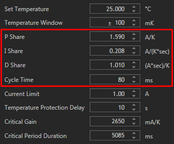
Figure 5.13 Final Calculated PID Parameters
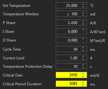
Figure 5.12 Entering the Critical Gain and Critical Period Duration
Alternatively, the PID parameters can be saved to the computer running the GUI. The next time that the GUI is used to operate the TEC driver, the saved parameters can be loaded into the GUI and will automatically populate all of the fields; the user can then select whether to save these parameters to the volatile memory only (meaning that the driver will immediately use the parameters), or to save the parameters to both the volatile and non-volatile memory.
Notes
The cycling time is the time basis of the internal digital control loop and is calculated automatically by entering the critical gain and the critical oscillation period. If the cycling time is manually reset, the firmware recalculates the I and the D shares.
The optimized PID parameters are valid for a steady state that is dependent on the set temperature as well as on the ambient conditions (ambient temperature, temperature of the thermally controlled object). Any changes in the operating and/or environmental conditions may require a re-adjustment of the PID parameters.
For more information on the basics of PID circuits, see the PID Tutorial tab.
PID Basics
The PID circuit is often utilized as a control loop feedback controller and is commonly used for many forms of servo circuits. The letters making up the acronym PID correspond to Proportional (P), Integral (I), and Derivative (D), which represents the three control settings of a PID circuit. The purpose of any servo circuit is to hold the system at a predetermined value (set point) for long periods of time. The PID circuit actively controls the system so as to hold it at the set point by generating an error signal that is essentially the difference between the set point and the current value. The three controls relate to the time-dependent error signal. At its simplest, this can be thought of as follows: Proportional is dependent upon the present error, Integral is dependent upon the accumulation of past error, and Derivative is the prediction of future error. The results of each of the controls are then fed into a weighted sum, which then adjusts the output of the circuit, u(t). This output is fed into a control device, its value is fed back into the circuit, and the process is allowed to actively stabilize the circuit’s output to reach and hold at the set point value. Figure 101A illustrates the action of a PID circuit. One or more of the controls can be utilized in any servo circuit depending on system demand and requirement (i.e., P, I, PI, PD, or PID).
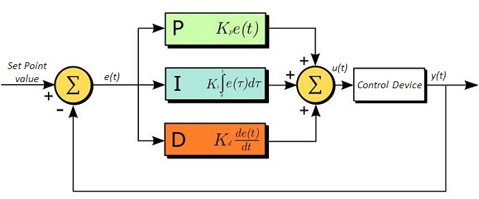 Figure 101A PID Diagram
Through proper setting of the controls in a PID circuit, relatively quick response with minimal overshoot (passing the set point value) and ringing (oscillation about the set point value) can be achieved. Let’s take as an example a temperature servo, such as that for temperature stabilization of a laser diode. The PID circuit will ultimately servo the current to a Thermoelectric Cooler (TEC) (often times through control of the gate voltage on an FET). Under this example, the current is referred to as the Manipulated Variable (MV). A thermistor is used to monitor the temperature of the laser diode, and the voltage over the thermistor is used as the Process Variable (PV). The Set Point (SP) voltage is set to correspond to the desired temperature. The error signal, e(t), is then the difference between the SP and PV. A PID controller will generate the error signal and then change the MV to reach the desired result. For example, if e(t) states that the laser diode is too hot, the circuit will allow more current to flow through the TEC (proportional control). Since proportional control is proportional to e(t), it may not cool the laser diode quickly enough. In that event, the circuit will further increase the amount of current through the TEC (integral control) by looking at the previous errors and adjusting the output to reach the desired value. As the SP is reached (e(t) approaches zero), the circuit will decrease the current through the TEC in anticipation of reaching the SP (derivative control).
Please note that a PID circuit will not guarantee optimal control. Improper setting of the PID controls can cause the circuit to oscillate significantly and lead to instability in control. It is up to the user to properly adjust the PID gains to ensure proper performance.
PID Theory
The output of the PID control circuit, u(t), is given as
where
Kp= Proportional Gain
Ki = Integral Gain
Kd = Derivative Gain
e(t) = SP - PV(t)
From here we can define the control units through their mathematical definition and discuss each in a little more detail. Proportional control is proportional to the error signal; as such, it is a direct response to the error signal generated by the circuit:
Larger proportional gain results in larger changes in response to the error, and thus affects the speed at which the controller can respond to changes in the system. While a high proportional gain can cause a circuit to respond swiftly, too high a value can cause oscillations about the SP value. Too low a value and the circuit cannot efficiently respond to changes in the system.
Integral control goes a step further than proportional gain, as it is proportional to not just the magnitude of the error signal but also the duration of the error.
Integral control is highly effective at increasing the response time of a circuit along with eliminating the steady-state error associated with purely proportional control. In essence integral control sums over the previous error, which was not corrected, and then multiplies that error by Ki to produce the integral response. Thus, for even small sustained error, a large aggregated integral response can be realized. However, due to the fast response of integral control, high gain values can cause significant overshoot of the SP value and lead to oscillation and instability. Too low, and the circuit will be significantly slower in responding to changes in the system.
Derivative control attempts to reduce the overshoot and ringing potential from proportional and integral control. It determines how quickly the circuit is changing over time (by looking at the derivative of the error signal) and multiplies it by Kd to produce the derivative response.
Unlike proportional and integral control, derivative control will slow the response of the circuit. In doing so, it is able to partially compensate for the overshoot as well as damp out any oscillations caused by integral and proportional control. High gain values cause the circuit to respond very slowly and can leave one susceptible to noise and high frequency oscillation (as the circuit becomes too slow to respond quickly). Too low and the circuit is prone to overshooting the SP value. However, in some cases overshooting the SP value by any significant amount must be avoided and thus a higher derivative gain (along with lower proportional gain) can be used. Table 101B explains the effects of increasing the gain of any one of the parameters independently.
| Table 101B PID Gain Parameter Effects | |||||
|---|---|---|---|---|---|
| Parameter Increased | Rise Time | Overshoot | Settling Time | Steady-State Error | Stability |
| Kp | Decrease | Increase | Small Change | Decrease | Degrade |
| Ki | Decrease | Increase | Increase | Decrease Significantly | Degrade |
| Kd | Minor Decrease | Minor Decrease | Minor Decrease | No Effect | Improve (for small Kd) |
Tuning
In general the gains of P, I, and D will need to be adjusted by the user in order to best servo the system. While there is not a static set of rules for what the values should be for any specific system, following the general procedures should help in tuning a circuit to match one’s system and environment. A PID circuit will typically overshoot the SP value slightly and then quickly damp out to reach the SP value.
Manual tuning of the gain settings is the simplest method for setting the PID controls. However, this procedure is done actively (the PID controller turned on and properly attached to the system) and requires some amount of experience to fully integrate. To tune your PID controller manually, first the integral and derivative gains are set to zero. Increase the proportional gain until you observe oscillation in the output. Your proportional gain should then be set to roughly half this value. After the proportional gain is set, increase the integral gain until any offset is corrected for on a time scale appropriate for your system. If you increase this gain too much, you will observe significant overshoot of the SP value and instability in the circuit. Once the integral gain is set, the derivative gain can then be increased. Derivative gain will reduce overshoot and damp the system quickly to the SP value. If you increase the derivative gain too much, you will see large overshoot (due to the circuit being too slow to respond). By playing with the gain settings, you can maximize the performance of your PID circuit, resulting in a circuit that quickly responds to changes in the system and effectively damps out oscillation about the SP value.
| Table 101C Control Circuit Gains | |||
|---|---|---|---|
| Control Type | Kp | Ki | Kd |
| P | 0.50 Ku | - | - |
| PI | 0.45 Ku | 1.2 Kp/Pu | - |
| PID | 0.60 Ku | 2 Kp/Pu | KpPu/8 |
While manual tuning can be very effective at setting a PID circuit for your specific system, it does require some amount of experience and understanding of PID circuits and response. The Ziegler-Nichols method for PID tuning offers a bit more structured guide to setting PID values. Again, you’ll want to set the integral and derivative gain to zero. Increase the proportional gain until the circuit starts to oscillate. We will call this gain level Ku. The oscillation will have a period of Pu. Gains for various control circuits are then given in Table 101C.
Note that when using the Ziegler-Nichols tuning method with some devices like the DSC1 digital servo controller, the integral and derivative terms must be normalized by the sample rate. To do this, the integral term determined from the table should be divided by the sample rate in Hertz and the derivative term should be multiplied by the sample rate in Hertz.
| Posted Comments: | |
user
(posted 2025-09-16 08:46:35.013) Hello,
I'm having an issue with the MTD1020T.
I'm sending commands via an UART to set all PID settings (T, W, L, d, G, O, P, I, D, C and S). The module acknowledges the values as expected.
The datasheet states that the "M" command triggers the saving of the current values to flash.
In my case, not all settings are saved to flash. The temperature target gets written, while the P share is never saved.
I'm testing without a temperature probe attached, which triggers the corresponding error flag, but no other error.
One hint about the issue, the "M" command returns 0/n after 5ms. This seems long, is this the expected reply? Am I to send the "M" command only once ? Any timings to be respected, that would not be specified in the datasheet?
Thanks for your answer. GBoedecker
(posted 2025-09-17 09:42:13.0) Thank you for your feedback! I tested it and the P setting was saved with the "M" command. I will contact you for troubleshooting. Stefano Bettelli
(posted 2025-06-04 08:51:26.753) Hallo, when using the GUI to the MTDEVAL1 board, is it possible to download the measured values (temperature and current) for offline analysis? GBoedecker
(posted 2025-06-04 09:25:07.0) Thank you for you feedback! In the software GUI you can save device settings and a screenshot, but not the temperature and current data. You can write your own application to accomplish this task, using the provided SDK. I will contact you to assist you further. 杨 若傲
(posted 2024-09-28 17:56:13.717) 最近测试了两块板,一块是连接数USB,电脑识别不了,还有一块是PID参数设置后,电流一直在高位(1A左右),即使是温度很接近的情况下,这两块板都无法实现控温。请问这个是什么情况? hkarpenko
(posted 2024-09-30 12:14:42.0) Dear customer,
thank you for your feedback. We will contact you directly to discuss this issue in detail with you. Peter Doherty
(posted 2024-02-18 12:29:56.707) If that TEC controller worked to control cooled sensors down to -20 C, I think that would make it even more useful.
Anyway to make it do that?
Thank you. hkarpenko
(posted 2024-02-20 11:24:39.0) Dear customer,
thank you very much for your feedback. I will forward your suggestion to our development team. Dietmar Fischer
(posted 2023-10-24 14:24:56.137) We have received a new batch of your MTD415T controllers. Surprisingly, they show a difference behavior than the controllers that we had ordered in 2021.
PID control for specific Coherent OPSL modules works fine with the controllers from 2021 but cannot leads to heavily oscillating temperatures for the 2023 batch. We used the same set of PID parameters for both modules and did tests for several OPSL modules and several MTD controllers.
What is the difference between 2021 and 2023 versions of your controllers? hchow
(posted 2025-03-12 09:05:39.0) Dear Mr. Fischer, thank you for your response. This is clearly a firmware issue. I will personally reach out to you to provide a solution. Daniel Mitrani
(posted 2023-08-31 11:26:25.697) I have an MTD415L module mounted in the MTD Evaluation Board. When testing it with the MTD Series software, I notice a couple of issues:
1) The current limit function does not work.
2) The polarity of the Peltier connection pins on the module is not in correspondence with the convention used by Peltier manufacturers. I.e., a current flowing from TEC+ (red cable) to TEC- (black cable) should cool the bottom side of the Peltier when observed with the red cable on the left side.
Could you please comment.
Best. jweimar
(posted 2023-09-04 09:25:59.0) Thank you very much for your feedback. Unfortunately, among TEC elements the naming of the TEC+ and TEC- is not consistent. This means that it is possible the MTD diver will cause the TEC element to heat instead of cooling when connected. I will contact you directly to provide further assistance. Frederik Schröder
(posted 2023-06-28 14:42:42.353) Hi, as already requested, I am wondering about the temperature range. Would it be possible to increase the temperature range of the MTD415T and the MTDEVAL1, ideally to -50 until 100 C? Thank you in advance! dpossin
(posted 2023-07-05 05:42:52.0) Dear Frederik,
Thank you for your feedback. Unfortunately we can´t offer an extended temperature range, since the built in thermistor doesn´t show a linear behaviour at those temperatures any more. The second reason why we can´t extend is that the ADC is not able to resolve a greater temperature range. I contact you directly to discuss this further. Berat Can Çekiç
(posted 2023-05-05 19:56:24.327) Hello,
We are using MTD1020T and getting unwanted data types such as -
- şşşşşşşşşşşşşşşşşşşşşşşşşşşşşşşşşşşşşşşşşşşşşşşşşşşşşşşşşşşşşşşşşşşşşşşşşşşşşşşşşşşşşşşşşşşşşşşşşşşşşşşşşşşşşşşşşşşşşşşşşøÈÂÀàøø€øäøòü€ü‚{FF}şüş{FF}à€äø€ÀÀ€²üàúÀ·üğžçüêûşüïşş{FF}€{FF}{FF}àòğàùÌøûğş‚Èüışşşşøş`ÂüşáüøüüòàøşşàşèğÄøüşøşüø€şÀğøüû€şøøÀüøÀøäşøüüşüıˆøşÀşüüüüÀüüıüøàøàøş{FF}ÀàÑúşøşòùø€ğşàÀàş‚€ğøàààøüÀøàşüüûğşğüà{FF}Øüøøü€üùşøüøğûüøòøøü{FF}{FF}úóøğàààùĞİøÅü€Àà -
The baud rate , data bits , stop and priority bits configurations have been done as its datasheet but still not getting proper commands . Im using USB-TTL convertor in order to Tx and Rx . How can we solve that problem ? GBoedecker
(posted 2023-05-08 10:07:53.0) Thank you very much for your feedback! Using the MTDEVAL1 evaluation board facilitates handling of the MTD1020T, since you can directly connect a standard USB cable. I will contact you directly about how to connect the MTD1020T with an adapter. Leonard Höck
(posted 2023-02-10 14:06:59.547) I just did a reset of the error register and now get the error code 17 when I check the register. Before the reset it was 0.
What does the error code 17 mean? I couldn't find anything in the data sheet. Thanks in advance wskopalik
(posted 2023-02-13 10:48:32.0) Thank you very much for your feedback!
The error register of the MTD415T chips has 16 bit and each bit indicates a different error event. If more than one error event occurs at the same time, the bits for each error event will be added, e.g. 17 corresponds to 1 + 16.
If you get the error code as a decimal number, it is usually best to convert it to a binary number. For 17 this would be 0000 0000 0001 0001. Then you can compare it to the error register in the data sheet. In this case, the bit numbers 0 and 4 are active (starting with 0 on the right) and set to 1 so these two errors are currently present on the system.
I will contact you directly to provide further assistance. user
(posted 2022-11-17 20:53:29.483) 15 TEC - TEC Element negative connection
Connect this pin to the positive terminal of the TEC element. 1
)
16 TEC + TEC Element positive connection
Connect this pin to the negative terminal of the TEC element. 1
) wskopalik
(posted 2022-11-18 03:31:41.0) Thank you very much for your feedback!
Unfortunately, the naming convention of the TEC+ and TEC- connections is not consistent among TEC elements. Therefore, it is in some cases necessary to reverse the polarity of the TEC connections to work properly with the MTD drivers.
I will contact you directly to provide further assistance. user
(posted 2022-11-16 10:05:25.49) I have a MTD415T, I have to reverse the TEC connections to make it to work.: pin-16 of MTD415T to pin-14 of SLD1005S (butterfly laser package);pin-15 to pin-1. what can be wrong? wskopalik
(posted 2022-11-18 03:13:30.0) Thank you very much for your feedback!
Unfortunately, the naming convention of the TEC+ and TEC- connections is not consistent among TEC elements. Therefore, it is in some cases necessary to reverse the polarity of the TEC connections to work properly with the MTD drivers.
I will contact you directly to provide further assistance. user
(posted 2022-06-28 01:42:20.713) Like others, I am very eager to extend the temperature limits of the MTD and MTD eval (e.g to -10 or colder). Is it possible to remove or edit the limit temperatures? hkarpenko
(posted 2022-07-01 06:10:21.0) Dear Alexander,
thank you for your interest in our products.
I am reaching out to you to discuss this further. Daniel Sablowski
(posted 2022-02-01 11:21:00.733) Dear Thorlabs-Team, is it possible to use TEC controller with higher currents (with heat sink) with your evaluation board? 10A would be my requirement. Thanks and best regards, Daniel soswald
(posted 2022-02-09 03:11:13.0) Dear Daniel,
thank you for your feedback. I have reached out to you directly to discuss your application in more detail and see if we can offer a suitable solution. C. Peppermueller
(posted 2021-12-06 11:32:45.99) We would like the MTD415L even more if it would allow a larger temperature range. Is there a way to extend the limit temperatures (5C, 45C)? We would love e.g. -5 to 70 C, or even hotter at the upper end. Is there a way to do that?
Thank you in advance,
Christian (Peppermueller) dpossin
(posted 2021-12-08 03:14:33.0) Dear customer,
Thank you for your feedback. I am reaching out to you in order to discuss this with you. Michael Levin
(posted 2021-06-07 23:53:12.06) Hi Thorlabs team,
I would like to make a remark regarding the output polarity of the MTD415T controller. A while ago, someone already asked this question (he had to revert the polarity while working with a butterfly laser). Your engineer replied that the actual polarity depends on how the TEC is mounted in the system. In general, this is correct.
But, practically, when you are working with a closed package (typically a laser or a detector, as in my case), the package pinout is so defined that positive voltage difference across its TEC results in cooling rather than heating of the active element. Therefore, in many applications (not to say in most), the TEC polarity is well-defined, and it would be nice if the output polarity of MTD415T were defined in just the same way, namely:
"The positive voltage difference between the TEC+ and TEC- terminals of the controller must result in cooling the active element to which the TEC is attached within the same package". I believe this is the natural way to define the output polarity of the controller, but unfortunately the actual polarity is reversed.
Another suggestion is to provide in the datasheet the value of the controller's efficiency, as this will help to choose the correct power supply for the controller. Now the datasheet only mentions "high efficiency", which is a not well-defined term.
Now I must say that the controller itself works very good, and my suggestions are only about the documentation.
Best regards,
Michael MKiess
(posted 2021-06-10 10:50:18.0) Dear Michael, Thank you very much for this feedback. Such suggestions for improvement can help us to better document our products, make them understandable and continuously improve them. We will address these points. Thank you for this helpful feedback. Christian Zingl
(posted 2021-05-25 05:34:15.747) There seems to be a problem using the MTD1020T on-board PID tuning algorithm. The sequence of sending the G and O commands determines whether or not the MTD1020T applies the PID coefficients.
I initially start with a MTD1020T with the PID and C parameters set to values not fitting my TEC system. Then I try to adjust the PID using the G and O commands.
There are two choices of sequencing when setting G and O:
- Apply power, then first send the G command, then the O command. Doing so results in oscillation or other unpredictable behavior as expected with wrong PID values
- Apply power, then first send the O command, then the G command. Now the PID controller works as expected.
Reading the P, I, D and C values returns the exact same values in both cases. It just seems that in one case, the values are not sent to the actual controller. This happens consistently over multiple retries with power cycles in between. MKiess
(posted 2021-05-28 06:42:58.0) Dear Christian, Thank you for your inquiry. I have contacted you directly to discuss the details and provide further support. Christian Zingl
(posted 2021-04-20 08:29:49.903) Dear Thorlabs Team,
it would be nice for the MTD1020T to support adjustable NTC coefficient with permanent storage (like for the PID settings).
Kind regards MKiess
(posted 2021-04-21 08:52:16.0) Dear Christian, Thank you for this feedback. Such feedback helps us to develop and improve our products. For these TEC drivers we also have the possibility to produce special designs with desired parameters for higher quantities.
A possible alternative would be our TED4015. Here you can e.g. set the NTC values as desired. Artem Gulyaev
(posted 2020-12-23 12:02:02.997) Hi,
Just for a bit convenience for the end user, could you please add in your datasheet that MTD415L answers for every "set" command with either
* corresponding value which was set
* with error message
surprisingly is was never declared in the datasheet, while is true.
Also probably error resetting mask also would be of some use - usually users might want to reset minor errors (like invalid value set attempt) while keeping the important ones. So "c" command might be accompanied with a mask value to erase.
Kind Regads,
Artem Gulyaev MKiess
(posted 2021-01-21 08:41:25.0) Thank you very much for this feedback. We will take a closer look at this topic again and see how we can make this more accessible to the end user, as described by you. Thank you very much for this suggestion. Such comments help us to constantly improve our products. Ludovic Angot
(posted 2020-07-23 07:43:40.233) I am currently writing my own code to use the MTDEVAL1 on a single board computer, the first step being a loopback test. To do so, can I safely only connect the USB cable and put a jumper on pins 12 and 13 (corresponding e.g. to TX and RX on the MTD1020) of either one of the carrier socket of the MTDEVAL1? Or does the evaluation board need to be powered via the Screw terminal 1 in order for the USB to UART to function? dpossin
(posted 2020-07-24 08:09:19.0) Dear Ludovic,
Yes, with no MTD module inserted you can use a jumper between pins 12 and 13 for the loopback test.
You don’t need to add an external power supply. user
(posted 2020-07-01 18:13:53.153) How many number of times can we program to the flash memory on MTD415T? Thank you. MKiess
(posted 2020-07-06 07:56:37.0) This is a response from Michael at Thorlabs. Thank you very much for your feedback. Depending on the application, more than 100k erase / write cycles are possible for the non-volatile memory (flash). We have the possibility to adapt the settings for your specific application to maximize the lifetime of the controller. I have contacted you directly to discuss this with you in more detail. user
(posted 2020-04-20 18:09:33.047) This is a nice product, I think two changes/variations would make it great.
1) A higher temperature version.
Many devices, such as doubling crystals, need to run at higher temps. I imagine you don't allow higher than +45 C because you cannot guarentee the ~ mK accuracy. For many applications ~ mK is not required. (For those out there who need a higher temp add a resistor to one of the sensor wires. The temp reading will no longer be accurate, and thorlabs specs won't hold at the higher real temp, but it works fine.)
2) compact version.
Although this is an eval board it would be quite useful if the footprint was reduced. It seems like it could be cut in half easily, maybe even by more with some effort. wskopalik
(posted 2020-04-21 11:57:11.0) This is a response from Wolfgang at Thorlabs. Thank you very much for your feedback!
We appreciate any feedback that helps us to improve our products. I will forward your suggestions to our engineering team so we can consider them for future releases in this product line. user
(posted 2019-10-23 08:32:31.37) The screw terminals for TEC+ and TEC- are too large to make proper contact with AWG 22 / 0.3 mm2 wires. The wire will be held in place barely, but will not have proper contact and can be pulled out by a little bit of force. Be sure to use suitable wires with larger cross sectional area to ensure proper contact.
The screw terminals for the power supply and sensor connection are both OK and don't have this issue. MKiess
(posted 2019-10-29 11:49:46.0) This is a response from Michael at Thorlabs. Thank you very much for your feedback. We appreciate any feedback that helps us to improve our products and helps all users to use them. user
(posted 2019-09-10 11:47:03.03) I'm controlling the PTC1 with my own SW via serial port according to the programmers reference of the MTD1020T, but I have encountered some communication problem.
The documentation is wrong, the Command/Response terminator is CR and not LF and each response value is followed by char '>' (62/0x3E). MKiess
(posted 2019-09-20 03:58:05.0) This is a response from Michael at Thorlabs. Thank you for the feedback. We will take a look at this and correct the documentation. Thank you very much for this information. Ludovic Angot
(posted 2019-07-29 22:40:27.34) I am planning to use the MTDEVAL1 on a linux system. I have already taken note of the programmer's reference of the TEC modules but there's nothing about UART control in the MTDEVAL1 manual. Could you please provide any guidelines to get me (and probably others) started on this? It may be as simple as connecting the eval. board, detecting the USB port and then send the appropriate commands, but I prefer to know beforehand to avoid any mistake. A short section on the topic could be added to the user manual. Also in paragraph 3 Operating Principle of the MTDEVAL1 manual, reference is made to saving the parameters to an XML file, could you provide an example of such an file? dpossin
(posted 2019-08-28 04:45:02.0) Dear Hinoki,
Thank you for your Feedback. The MTD Series uses standard serial communication over a virtual COM port for data transfer.
To control one of our MTD modules with a Linux based system you just need to use the operating system proprietary serial communication interface and you can use the standard commands mentioned in the manual.
I hope that helps. user
(posted 2019-07-09 17:16:26.473) Hi, is there a way to change the y-axis range in the MTD software? If my set temperature is 25 C, can I set the temperature range in the y-axis to 25+- 0.1C or something else? dpossin
(posted 2019-07-17 08:25:15.0) Dear customer,
Thank you for your feedback. You can adjust the viewing range of the temperature graph by setting the range on the left hand side by setting the desired range in the field "Temperature Window". Ingo Gersonde
(posted 2019-03-26 05:01:19.65) I use the MTD415TE on an evaluation board, applied to TEC and thermistor of a laser head. When i use the D_Share value, i get severe noise on the TEC current. Can one filter the temperatur signal or the TEC-output signal ?
Thank you in advance
Ingo Gersonde swick
(posted 2019-03-26 09:19:15.0) This is a response from Sebastian at Thorlabs. Thank you for the feedback.
The noise on TEC current could be caused by unshielded cables for the signal from Thermistor or D-Share value is set too high. In first case noise in sub-mV regime triggers D-share and in second case the value of D-share is too high in respect to P and I share. For improved noise immunity signals should be guided in shielded and twisted cables with reduced length. If PID values are not optimal please follow our guideline on the website at tab "PID Oscillation Test" or in the manual chapter 7.
I contacted you directly for further troubleshooting. Matthias.Nagel
(posted 2018-08-06 15:53:41.887) Can I drive 2 x ET-031-10-20 with the MTD1020T and th evaluation board? nreusch
(posted 2018-08-08 08:37:51.0) This is a response from Nicola at Thorlabs. Thank you for your inquiry. I checked the voltage and current requirements of the Peltier element you mentioned: Maximum current is 2.5 A and maximum voltage 3.8 V. Therefore, you should be able to drive two elements in a series connection since the voltage drop across two elements is 7.8 V, i.e. lower than the specified 10 V for MTD1020T. Please note that the maximum output current of MTD1020T is 2.0 A, so it will not allow you to drive the elements at their maximum current. The recommended TEC elements for this driver are TECH3S, TECL4 and TECJ6. I will contact you directly to discuss further details of your specific application. ward.becelaere
(posted 2018-04-11 15:43:46.01) According to the specs, the temperature range is between 5 and 45 C.
For my application I need a range between 15 and 75 C. Is there any way to have an extended range? Maybe a different thermistor?
Thanks! swick
(posted 2018-04-17 03:56:10.0) This is a response from Sebastian at Thorlabs. Thank you for the inquiry. For OEM applications we offer customizations suitable to a wide range of requirements. Customization of the MTD1020T for an other temperature range is possible. We contacted you directly for further discussion. xjiang225
(posted 2017-12-01 23:46:02.757) I have installed the MTD software but could not find the device in the software("Scan USB" doesn't give any result). I can see the device as both COM port and USB port in device manager. The "POWER SUPPLY" LED3 is the only LED that is on on the board. Could you please suggest some possible issues that are causing this? Thanks! swick
(posted 2017-12-05 04:33:13.0) This is a response from Sebastian at Thorlabs. Thank you for the inquiry. I have contacted you directly for troubleshooting. user
(posted 2017-11-15 09:58:43.903) Can you share more information about the thermistor readout circuit; as well as the expected thermistor B constant?
I need to design an interface circuit so that I can use a different type thermistor (R=9kOhm, B=~3400K) mvonsivers
(posted 2017-11-21 03:29:16.0) This is a response from Moritz at Thorlabs. Thank you for your inquiry. Unfortunately, MTD415T can only be used with 10 kOhm thermistors. However, the MTD-Modules can be customized for high quantity orders. Please contact techsupport@thorlabs.com for further information. mvonsivers
(posted 2017-11-22 03:59:56.0) This is a response from Moritz at Thorlabs. Our engineers have found a workaround for your problem. You can connect your 9 kOhm thermistor directly to the MTD415T module. In this case, you will get an offset between real temperature and read out value. This offset has to be taken into account when setting the set temperature.
Our MTD modules are calibrated for a B constant [25/85°C] = 3950 K. Your slightly different B constant will lead to a non-linearity over the complete temperature range. If your application requires only temperature stabilization at one operating point you should still be able to find the right PID parameters.
As already mentioned, for an OEM application we can modify and calibrate the MTD module according to your specifications. rogier
(posted 2017-09-29 17:38:09.133) Hello,
It seems that your current manual is not up-to-date. The programmers reference is saying that you should use quotations marks around the commands it seems with the new firmware update (1.0.5) on the MTD1020T this is no longer needed. The response isn’t written in brackets either as suggest in the manual. swick
(posted 2017-10-05 03:33:56.0) This is a response from Sebastian at Thorlabs. Thank you for the inquiry.
In the manual at chapter 5.1 you can find the nomenclature used for this device. The quotation marks or brackets are not part of the command or received message. This nomenclature makes it easier to distinguish between commands, received messages and formats.
I will contact you directly for further assistance. chkwak
(posted 2017-08-11 15:07:47.68) Hello
I buyed MTD415TE,
but this error message occur frequently,
"TEC current was too long time on the limit without influence on the temperature."
Let me know how to fix it. mdiekmann
(posted 2017-08-16 10:58:42.0) This is a response from Meike at Thorlabs: Thank you for contacting us! This error typically indicates that the thermal load is too large for the module to handle. It is a safety feature to prevent the unit from overheating. We will contact you directly to troubleshoot the issue in your case. slawomir.drobczynski
(posted 2017-07-17 00:38:43.053) I am using MTD415T and I would like to increase temperature from 25 to 36 degrees of Celsius. I start with factory default settings, why after few seconds TEC current is zero and Error Register: Thermal Latch-Up (TEC current at limit without temperature improvement) ? wskopalik
(posted 2017-07-20 06:01:23.0) This is a response from Wolfgang at Thorlabs. Thank you very much for your feedback.
Our MTD modules have a wide variety of safety features which can be en- or disabled by the costumer if needed.
The ”Thermal-Latch-Up Error” prevents the cooling system from over-heating. The module measures the output power of the module and if no change in terms of TEC temperature is recognizable, the module switches the output off to prevent the system from over-heating.
This can e.g. happen for very large thermal loads, because the change in temperature will happen very slow in this case. Please consider that the MTD415T is not designed to drive very large thermal loads. In normal operation this safety feature should not be triggered.
As a workaround for your application, you could disable the corresponding safety bitmask. You need to send the command "S251" over a terminal program to the module for this.
I will contact you directly to provide further assistance. krevety
(posted 2017-06-14 09:31:07.563) Are you planning a replacement for MTDEVAL?
btw. Excellent product, I like the MTD control app. tcampbell
(posted 2017-06-16 10:42:16.0) Response from Tim at Thorlabs: Thank you for your feedback. Yes, we have been developing a replacement for the MTDEVAL and it should be available for purchase shortly. j.zeludevicius
(posted 2017-01-06 05:28:39.763) I would like to express my two issues with MTDEVAL board and MTD415TE controller.
I used this controller for temperature stabilization of pump laser diode in 14-pin butterfly package. Controller board was connected to NTC 10K thermistor and TEC. When I connected TEC leads correctly (+ to +, and - to -) I got erroneous behavior of the controller. It decreased temperature (up to minimum value) when the temperature had to be increased. I reversed TEC connection polarity and then It worked correctly. Could you check whether there is any error in controller design?
Second issue is with operation status LED. When USB cable is disconnected the status LED turns off and it is not clear whether temperature control is active or is switch off as well. Could you comment on that? I have observed that status LED lights up whenever USB cable is connected to any source providing +5V, not necessary a computer. swick
(posted 2017-01-09 04:16:46.0) This is a response from Sebastian at Thorlabs. Thank you very much for the feedback.
Your description is exactly how the MTD modules are designed to work, your MTD module and the Evaluation board are working fine.
Let me explain this in more detail:
TEC:
The described behavior, that you need to change the polarity of the TEC element is based on the mounting direction of your TEC element. You can change hot and cold site by changing the polarity of the lead wires or by changing the mounting direction of the TEC element itself. Please be aware, that Thorlabs cannot predict the mounting direction of each TEC element, so by changing the polarity of the lead wires you have the maximum flexibility.
For your information: By using the MTD Software you will get an error code, which describes if the TEC element is connected in the wrong way.
LED:
Please refer to the manual for the function of the LED. The LED describes not if the MTD module is en- or disabled. It signals if the temperature is within the programmed temperature window. This is a very helpful feature to interface other (analog) circuitry to get a “Temperature Ready Signal”.
To use this function correctly we recommend to adjust the “Temperature Window” and the “Temperature Protection Delay” in the right way.
I will contact you directly for further assistance. gtoner2506
(posted 2016-12-21 05:05:49.833) I need to talk to this device using an embedded processor. Is ther a serial command set for it? wskopalik
(posted 2016-12-22 08:09:50.0) This is a response from Wolfgang at Thorlabs. Thank you for your inquiry.
These termperature controllers have an UART programming interface. A list of commands can be found in the manual from p.12 on.
I will contact you directly to discuss your application in more detail. cbrideau
(posted 2016-12-06 14:37:03.893) That was quick! The eval board looks great: Next challenge is to put connectors on this eval board and the LD eval board so you can put them together in a stack and share power supplies. swick
(posted 2016-12-07 03:17:26.0) This is a response from Sebastian at Thorlabs. Thank you for the feedback. We will discuss your suggestion in our internal forum. cbrideau
(posted 2016-11-30 15:51:30.177) Would be nice to see a daughter board and evaluation board for these like the MLD203 series laser drivers. An evaluation board that sockets one of the MLD203's AND one of these temperature controllers would be very handy for proto builders and evaluating the performance of the controllers. tfrisch
(posted 2016-12-02 02:42:40.0) Hello, thank you for contacting Thorlabs. I have posted this in our internal engineering forum. |

 Zoom
Zoom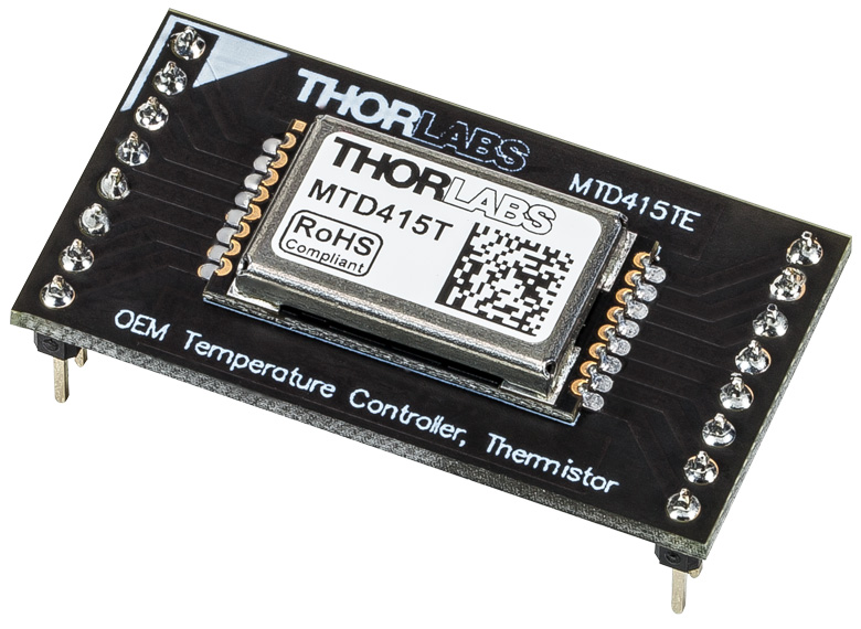
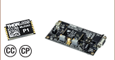
Click to Enlarge
Figure G1.1 MTD415TE TEC Driver on Daughterboard
- MTD415 Series in SMT Packages and on Daughterboards
- MTD1020T in a THT Package
- Daughterboard and THT Packages Mount Directly on the MTDEVAL1 Evaluation Board (Available Below)
- Supported Temperature Sensor Options
- 10 kΩ Thermistor
- LMT84 IC
- Control via Command Line or GUI (See Software tab)
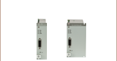
MTD415 Series
The MTD415 TEC controllers are available as either 16-pin surface-mount technology (SMTs) packages or with this package mounted on a daughterboard. The low thermal dissipation of the MTD415 Series minimizes the need for external components such as a heat sink. The compact 21.0 mm × 12.4 mm × 3.1 mm form factor of the SMT package uses plated half-hole connectors to allow easy surface mounting and electrical connections. The daughterboard serves as an adapter board for the SMT packages and mounts directly on the MTDEVAL1 evaluation board, which is offered below.
These TEC controllers deliver powers up to 6 W and a maximum TEC current of ±1.5 A. The MTD415L(E) supports the LMT84 IC temperature sensor, and the MTD415T(E) supports a 10 kΩ thermistor. Please see the Specs tab for plots showing the dependence of the output power and current on the load resistance. Pinout diagrams and typical application circuits are included in the Pin Diagrams tab.
MTD1020T
The MTD1020T is offered in a through-hole technology (THT) package with an integrated heatsink. This package both enables integration into PCBs and is directly compatible with a set of sockets on the MTDEVAL1 evaluation board. For optimal operation, we recommend actively cooling the MTD1020T when ambient temperatures exceed 20 °C.
The MTD1020T TEC controller delivers power up to 20 W. A maximum TEC current of ±2.0 A is delivered into any load resistance up to 5 Ω when operating under recommended conditions and adequately cooled. Please see the Specs tab for plots of the dependence of the output power on load resistance and cooling conditions, as well as a plot of the delivered current on cooling conditions. The MTD1020T supports a 10 kΩ thermistor. Pin out diagrams and a typical application circuit using the MTD1020T can be found in the Pin Diagrams tab.
Volume Pricing
Volume pricing is available for these TEC drivers. To view our current price schedules, please click the "Volume Pricing" links located below. Upon request, large-quantity orders of our MTD415 Series drivers can be delivered in an IC tube for simplified integration with assembly equipment.
| Item #a | Supported Temperature Sensor | TEC Compliance Voltage | Output Current (Max) | 16 Pin Package Type | Mounts on Evaluation Board | Recommended TEC |
|---|---|---|---|---|---|---|
| MTD415L | LMT84 IC | 4.0 V | ±1.5 A | SMTb | No | TECF2S, TECH4 |
| MTD415LE | LMT84 IC | 4.0 V | ±1.5 A | Daughterboard | Yes | |
| MTD415T | 10 kΩ Thermistor | 4.0 V | ±1.5 A | SMTb | No | |
| MTD415TE | 10 kΩ Thermistor | 4.0 V | ±1.5 A | Daughterboard | Yes | |
| MTD1020T | 10 kΩ Thermistor | 10.0 V | ±2.0 A | THTc | Yes |

 Zoom
Zoom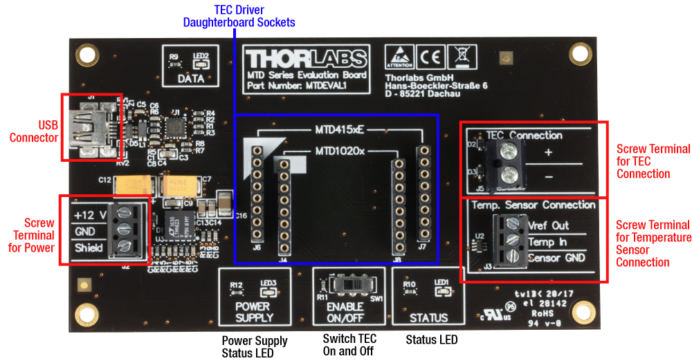
Click to Enlarge
Figure G2.2 Evaluation Board with MTD415LE TEC Driver Installed
- Outer Socket Mounts the MTD415LE and MTD415TE Daughterboards
- Inner Socket Mounts the MTD1020T THT Package
- Screw Terminals for:
- 12 VDC, 2.3 A Power Supply
- TEC Connections
- Temperature Sensor Connections
- USB Connector for Control via GUI (See Software Tab)
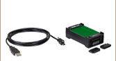
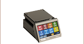
Evaluation Board
The MTDEVAL1 Evaluation Board is a break-out board that allows our OEM-grade TEC drivers (available above) to be quickly deployed in laboratory and test environments. The MTDEVAL1 facilitates PC control of the TEC Driver as well as connections to 12 V power, the TEC, and a temperature sensor. To enable computer control of the mounted driver first use a compatible cable, such as the USB-AB-72 (available below), to connect the PC to the 2.0 USB type Mini B port on the MTDEVAL1. When the evaluation board is connected to a computer, the settings of the mounted TEC driver can be changed using either text commands sent over UART, which are outlined in the data sheet, or through the MTD GUI available on the Software tab. In addition to allowing users to manually set the parameters of the control loop, the GUI can calculate the optimal P, I, and D parameters using the results of an oscillation test (see the PID Oscillation Test tab for details). When getting started, install the driver software before connecting the MTDEVAL1 to a PC; installing the driver software after connection can cause errors in the installation.
For autonomous operation of the TEC driver, it is not necessary to connect the evaluation board to a computer. When power is supplied to the board, TEC and temperature sensor wires are connected to the appropriate screw terminals, and the SW1 (ENABLE ON/OFF) switch s set in the on position, the TEC driver will operate according to the settings saved to its flash memory.
Compatible TEC Drivers
The MTD1020T TEC driver has pins that allow it to be mounted using the inner socket on the MTDEVAL1 board. The MTD415 Series TEC drivers include daughterboard configurations, the MTD415LE and MTD415TE, in which the surface-mount technology (SMTs) packages are mounted on an adapter board, that are compatible with the outer mounting sockets on the evaluation board.
To protect the TEC driver from potential electrical damage, ensure that power is disconnected from the evaluation board when installing the TEC driver on the MTDEVAL1. Please note that setting the SW1 (ENABLE ON/OFF) switch to the off position does not disconnect power from the sockets. Instead, SW1 is used to enable or disable the TEC driver's control of the connected TEC. The SW1 switch should be set to the off position prior to supplying power to the board.