 Products Home
Liquid Crystal Polarization Rotators
- Smooth and Continuous Rotation of Linear Input Polarization
- Compact Design with >1000:1 Extinction Ratio
- 532 or 633 nm Design Wavelength Available from Stock
- Custom Versions with Design Wavelengths from 400 to 1700 nm
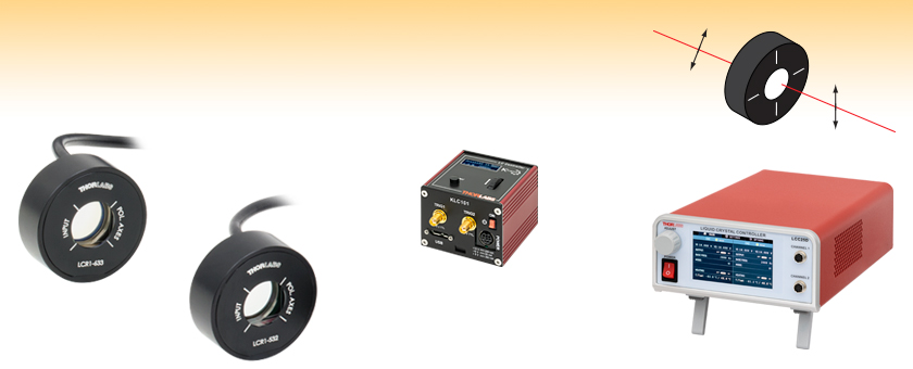
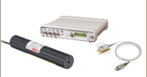
LCR1-633
633 nm Polarization Rotator
LCR1-532
532 nm Polarization Rotator
Input Polarization
Output Polarization
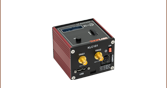
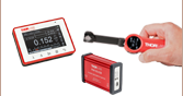
KLC101
K-Cube® LC Controller
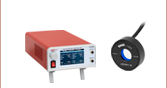
LCC25D
2-Channel
Benchtop LC Controller


Please Wait
| Item # | LCR1-532 | LCR1-633 | |
|---|---|---|---|
| Operating Wavelength | 532 nm | 633 nm | |
| Clear Aperture | 10 mm | ||
| Thickness | 9.4 mm | ||
| AR Coating |
Input Side | Ravg < 0.5% from 350 to 700 nm | |
| Output Side | R < 0.25% at 532 nm (V-Coat) |
R < 0.25% at 633 nm (V-Coat) |
|
| Extinction Ratioa,b | >1000:1 | ||
| TWEc | λ/4 at 635 nm | ||
| Surface Quality | 40-20 Scratch Dig | ||
| Angle of Incidence | <1.5° | ||
| Rotation Angle | -90° to +90° (>180° of Rotation) | ||
| Damage Threshold | 1.0 J/cm2 (532 nm, 10 Hz, 8 ns, Ø200 µm) 0.01 J/cm2 (532 nm, 100 Hz, 76 fs, Ø162 µm) |
||
Features
- Rotate Linear Input Polarization Continuously Through >180°
- Extinction Ratio: >1000:1
- AR Coatings on Air-to-Glass Interfaces
- 532 nm or 633 nm Operating Wavelength from Stock
- Other Wavelengths Available by Contacting Tech Support
Thorlabs' Liquid Crystal (LC) Polarization Rotators can continuously rotate the polarization state of a linearly polarized input beam through more than 180° with no mechanical movement involved. A minimum extinction ratio of 1000:1 is guaranteed over the entire rotation range.
An LC polarization rotator consists of a liquid crystal variable retarder and a quartz zero-order quarter-wave plate; the LC retarder and wave plate have their fast axes oriented at 45° with respect to each other, as shown in Figure 1.1. With linearly polarized light incident on the polarization rotator from the liquid crystal cell side, azimuth rotation of the output polarization can be achieved by adjusting the liquid crystal retardation. The input beam should be linearly polarized with the polarization direction aligned with one of the rotator input axes (marked on the front of the housing).
All liquid crystal polarization rotators are tested at the design wavelength before shipment. The output rotation versus control voltage curve for continuous rotation from -90° to +90° (at least 180° of rotation) is shipped with each device.
Click to Enlarge
Figure 1.1 A Schematic Showing the Operating Principle of the LC Polarization Rotator
Operating Principle
As shown in Figure 1.1, the input polarization should be aligned to either Axis 1 or Axis 2, as marked by the engraved lines on the front of the housing. In this orientation, the input polarization state is at a 45° angle to the fast and slow axes of the LC retarder. The difference in retardance between the fast and slow axes of the LC retarder converts the linear input polarization into an elliptical polarization that has its major and minor axis oriented at 45° with respect to the fast and slow axes of the LC retarder. The amount of ellipticity will vary depending on the phase difference between the fast and slow axes.
The quarter-wave plate is aligned so that its fast and slow axes are also at a 45° angle with respect to the fast and slow axes of the LC retarder; as a result, the elliptical polarization that exits the LC retarder will be converted back to a linear polarization by the quarter-wave plate, while the angle of the output linear polarization will be dependent on the ellipticity produced by the LC retarder.
We also offer a Deterministic Polarization Rotator that incorporates a closed-loop feedback system to stabilize the output azimuth for applications requiring precise and stable linear polarizations.
Voltage Controllers
The LCC25, LCC25D, and KLC101 liquid crystal controllers provide active DC offset compensation while applying an AC voltage (0 to 25 Vrms). The DC offset compensation automatically zeros the DC bias across the LC device in order to counteract the buildup of charge.
Performance
Our liquid crystal polarization rotators are each designed to operate at a specific wavelength. We provide polarization rotation data for each polarization rotator at its design wavelength with the input rotation set at 0° (horizontal). Additionally, the output beam polarization extinction ratio (ER) versus input wavelength shift is shown in Figures 2.3 and 2.6. As input wavelength shifts away from the design wavelength, the output beam ER decreases. The data shown shows measurements for both alignment axes of the rotator, but only one is used during operation. All tests were obtained at the design wavelength using a LCC25 liquid crystal controller and a LPVISE100-A polarizer at the input.
LCR1-532 Rotation Angle, Extinction Ratio, and Control Voltage

Click to Enlarge
Click Here for Raw Data
Figure 2.1 This data was taken with 0° (horizontal) input polarization. The vertical dashed lines mark the control voltages corresonding to 90°, 0°, and -90°.
Click to Enlarge
Click Here for Raw Data
Figure 2.2 This plot shows the calculated ER based on the measured ellipticity, where ER = [tan(ellipticity)]-2. The data was taken with the input polarization precisely aligned to 0°, allowing the LCR1-532 to achieve ER > 1000:1 over the entire working control voltage range.
Click to Enlarge
Click Here for Raw Data
Figure 2.3 The ER of the output light will decrease as the input wavelength deviates from the design wavelength. The ER data used in this plot for each wavelength is the lowest achievable ER for that wavelength.
LCR1-633 Rotation Angle, Extinction Ratio, and Control Voltage
Click to Enlarge
Click Here for Raw Data
Figure 2.4 This data was taken with 0° (horizontal) input polarization. The vertical dashed lines mark the control voltages corresonding to 180°, 90°, 0°, and -90°.
Click to Enlarge
Click Here for Raw Data
Figure 2.5 This plot shows the calculated ER based on the measured ellipticity, where ER = [tan(ellipticity)]-2. The data was taken with the input polarization precisely aligned to 0°, allowing the LCR1-633 to achieve ER > 1000:1 over the entire working control voltage range.

Click to Enlarge
Click Here for Raw Data
Figure 2.6 The ER of the output light will decrease as the input wavelength deviates from the design wavelength. The ER data used in this plot for each wavelength is the achievable ER for that wavelength.
Angle of Incidence
These LC Polarization Rotators are sensitive to the angle of incidence (AOI). Figures 2.7 and 2.8 show the effect of AOI on the output beam rotation: an AOI <±1° is required to keep the change in output rotation angle within 3°.
Click to Enlarge
Click Here for Raw Data
Figure 2.7 Change in the polarization rotation angle as the incident angle is changed from -8° to 8°. The rotator was set to produce an output polarization parallel to the input polarization when the AOI was 0°.
Click to Enlarge
Click Here for Raw Data
Figure 2.8 Change in the polarization rotation angle as the incident angle is changed from -8° to 8°. The rotator was set to produce an output polarization parallel to the input polarization when the AOI was 0°.
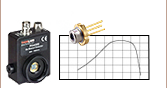
Transmission
To improve transmission through the device, both the LCR1-532 and LCR1-633 have a broadband AR coating on one outer optic surface (Ravg < 0.5% from 350 to 700 nm) and a V-Coat centered on the design wavelength on the other outer optic surface (R < 0.25% at design wavelength). Figures 2.9 and 2.10 show typical transmission curves for these two rotators.
Click to Enlarge
Click Here for Raw Data
Figure 2.9 Typical Transmission of LCR1-532 Polarization Rotator

Click to Enlarge
Click Here for Raw Data
Figure 2.10 Typical Transmission of LCR1-633 Polarization Rotator
Click to Enlarge
Figure 3.1 Switching time for LCR1-532 measured at 23 °C. Switching times for different modes are indicated by different colors. Solid lines indicate fall times and dashed lines indicate rise times.
LC Polarization Rotator Switching Time
Liquid crystal polarization rotators feature a short switching time compared to mechanical variable wave plates due to the lack of moving parts. The switching time of a liquid crystal polarization rotator depends on several variables, some of which are controlled in the manufacturing process, and some by the user. An example of switching times for a single polarization rotator is shown in Figure 3.1.
In general, liquid crystal polarization rotators will always switch faster at higher driving voltage than at lower driving voltage. Also, the fall time (from low voltage to high voltage) is faster than rise time (from high voltage to low voltage) when the LC polarization rotator is switched between two voltages.
In addition, the material's viscosity and hence the switching speed also depend on temperature of the LC material. As can be seen in Tables 3.2 and 3.3, the switching speed can increase by as much as two times by heating the LC polarization rotator. Our standard LC polarization rotators are designed to work at temperatures up to 45 °C, where they can still maintain the specified rotation. If additional speed is required, the polarization rotators can work at temperatures up to 70 °C, but the maximum retardation value will be lower.
The switching speed is also related to the thickness of the LC polarization rotator, the rotational viscosity of the LC material, and the dielectric anisotropy of the LC material. However, since each of those variables affects other operating parameters as well, our LC polarization rotators are designed to optimize overall performance, with a special emphasis on switching time. We also offer custom and OEM LC polarization rotators optimized for other parameters, as well as faster liquid crystal rotators. See the Custom Rotators tab, or contact techsupport@thorlabs.com for details.
Switching Times
Typical rotator switching times are shown here for three typical output rotations and four temperatures.
| Table 3.2 LCR1-532 Switching Times | |||||
|---|---|---|---|---|---|
| Switching Mode | V1 | V2 | Temperature | Rise Timea | Fall Timeb |
| 90° and 0° | 0.99 V | 1.56 V | 23 °C | 85.00 ms | 73.75 ms |
| 45 °C | 79.75 ms | 43.70 ms | |||
| 60 °C | 77.25 ms | 33.25 ms | |||
| 70 °C | 78.00 ms | 26.75 ms | |||
| 90° and -90° | 0.99 V | 2.67 V | 23 °C | 81.75 ms | 21.25 ms |
| 45 °C | 66.00 ms | 8.25 ms | |||
| 60 °C | 65.75 ms | 8.25 ms | |||
| 70 °C | 64.25 ms | 5.25 ms | |||
| 0° and -90° | 1.56 V | 2.67 V | 23 °C | 37.25 ms | 15.00 ms |
| 45 °C | 33.50 ms | 5.00 ms | |||
| 60 °C | 25.25 ms | 5.50 ms | |||
| 70 °C | 22.00 ms | 4.75 ms | |||
| Table 3.3 LCR1-633 Switching Times | |||||
|---|---|---|---|---|---|
| Switching Mode | V1 | V2 | Temperature | Rise Timea | Fall Timeb |
| 90° and 0° | 1.28 V | 1.68 V | 23 °C | 122.00 ms | 103.00 ms |
| 45 °C | 118.50 ms | 66.50 ms | |||
| 60 °C | 108.25 ms | 51.50 ms | |||
| 70 °C | 78.50 ms | 39.25 ms | |||
| 90° and -90° | 1.28 V | 2.71 V | 23 °C | 130.75 ms | 31.75 ms |
| 45 °C | 108.50 ms | 14.00 ms | |||
| 60 °C | 88.00 ms | 8.75 ms | |||
| 70 °C | 83.25 ms | 5.75 ms | |||
| 0° and -90° | 1.58 V | 2.71 V | 23 °C | 75.25 ms | 25.25 ms |
| 45 °C | 56.25 ms | 10.25 ms | |||
| 60 °C | 42.75 ms | 4.75 ms | |||
| 70 °C | 40.25 ms | 11.00 ms | |||
Click to Enlarge
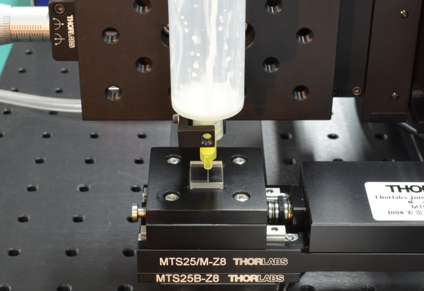
Figure 4.1 The LC Polarization Rotator should be aligned using two crossed polarizers following the steps outlined in this tab.
Alignment
In order to precisely align the axis of the liquid crystal polarization rotator, mount the rotator in an appropriate rotation mount (RSP1(/M) or the CRM1PT(/M) recommended). Then set up a detector or power meter to monitor the transmission of a beam through a pair of crossed linear polarizers. The input polarization should have an extinction ratio of at least 1000:1. Fine alignment for the LC rotator is accomplished using the following procedure:
- Place the LC polarization rotator between two crossed polarizers with one of its input axes roughly aligned with the transmission axis of the first polarizer.
- Using the LCC25, LCC25D, or KLC101 controller (or equivalent), apply the control voltage corresponding to zero degrees of rotation for the LC rotator (see the product report included in each package).
- Use the rotation mount to turn the LC polarization rotator slowly until the transmitted intensity is minimized. Then fine tune the control voltage to further reduce the transmitted power intensity.
- Repeat step 3 at least three times to ensure that the LC rotator is properly aligned with first linear polarizer.
- Remove second linear polarizer and power meter. The polarization rotator is now ready for use.
Custom Capability
In addition to our standard liquid crystal (LC) polarization rotators that provide >180° continuous rotation and a Ø10 mm clear aperture, Thorlabs can also produce custom and OEM rotators. The rotation range, coating, temperature stabilization, and dimension can be customized to meet many unique optical designs. We also offer other custom liquid crystal devices, such as empty LC cells, liquid crystal variable retarders, and noise eaters. For more information about ordering a customized liquid crystal device, please contact Thorlabs' Tech Support.
Our engineers work directly with our customers to discuss the specifications and other design aspects of a custom liquid crystal device. They will analyze both the design and feasibility to ensure the custom products are manufactured to high-quality standards and in a timely manner.
Liquid Crystal Polarization Rotator Manufacturing
- Coating Glass Substrates with the Alignment Layer: Glass substrates are spin coated with a Polyimide (PI) solution. Then the coated substrate is baked at 250 °C so that the PI solution forms a thin film of alignment layer on the substrate.
- Rubbing: A mechanical rubbing process is employed on the alignment layer. The micro-fiber on the rubbing cloth creates fine scratches on the alignment layer surface, which defines alignment direction and pre-tilt angle of liquid crystal molecules.
- Drawing Sealant Lines on the Glass Substrates: Thermal sealant mixed with spacer particles is drawn into a frame around the clear aperture, determining the cell gap of the liquid crystal (LC) cell.
- Coupling of Glass Substrates and Sealant Curing: Two glass substrates are coupled into a cell, and then the thermal sealant is baked into rigid solid lines.
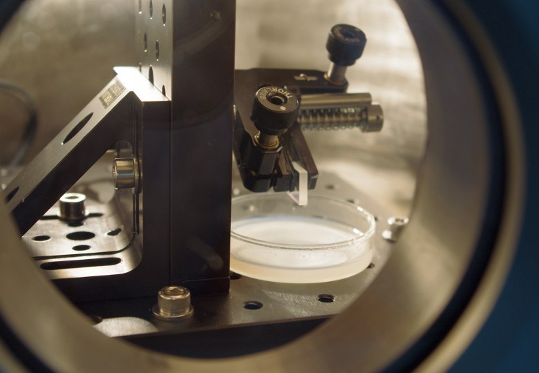
- Filling the Cell with Liquid Crystal: The empty cell is filled with liquid crystal while in a vacuum chamber, preventing air bubbles or dust from contaminating the LC. The opening in the sealant line is then sealed with glue.
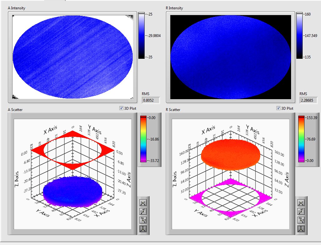
- Retardance-versus-Voltage Uniformity Test: The voltage-retardation (RV) characteristics of each LC cell are tested.
- A Quartz Quarter Wave Plate is bonded onto the LC cell to complete the polarization rotator. The fast axis of the compensator is 45° to that of the LC retarder.
- Final Rotation versus Control Voltage and ER versus Control Voltage Test: The voltage versus rotation and voltage versus ER characteristics of each rotator are tested and recorded for the test report included in package.
- Assembly into Housing and Circuit Calibration (If Applicable): The LC polarization rotator is assembled into mechanical housing, which is compatible with Thorlabs' standard 1" or 2" mounts. The driving circuit can also be mounted into the housing and calibrated.
| Table 5.3 Polarization Rotator Customization Options | |
|---|---|
| Feature | Specification |
| Rotator Thickness (without Mechanical Housing) |
4 - 12 mm |
| Operating Wavelength | 400 - 2020 nm |
| Continuous Rotation Range | 0° - 1800° |
| AR Coating | Wavelengths from 400 to 2020 nm |
| Clear Aperture | ≤Ø2" |
| Other Features | Mechanical Housing Phase Compensator Temperature Control Integrated Control Unit |
Customizable Features
Table 5.3 outlines LC polarization rotator features that can be customized. For specifications outside of the listed ranges, please contact Tech Support.
Thinner glass substrates enable more compact LC cells to be used in the rotator, at the cost of being easier to bend. Therefore, we recommend using thicker glass substrates for better consistency in the uniformity of the retardation.
We encourage customers to contact our Tech Support team and discuss their specific requirements for customized liquid crystal retarders. Our Tech Support and engineering teams will work together to make sure that our customers receive devices optimized to meet their requests.
| Table 6.1 Damage Threshold Specifications | ||
|---|---|---|
| Item # | Laser Type | Damage Threshold |
| LCR1-532 | Pulsed (ns) | 1.0 J/cm2 (532 nm, 10 Hz, 8 ns, Ø200 µm) |
| Pulsed (fs) | 0.01 J/cm2 (532 nm, 100 Hz, 76 fs, Ø162 µm) | |
| LCR1-633 | Pulsed (ns) | 1.0 J/cm2 (532 nm, 10 Hz, 8 ns, Ø200 µm) |
| Pulsed (fs) | 0.01 J/cm2 (532 nm, 100 Hz, 76 fs, Ø162 µm) | |
Damage Threshold Data for Thorlabs' Liquid Crystal Polarization Rotators
The specifications in Table 6.1 are measured data for Thorlabs' Liquid Crystal Polarization Rotators.
Laser Induced Damage Threshold Tutorial
The following is a general overview of how laser induced damage thresholds are measured and how the values may be utilized in determining the appropriateness of an optic for a given application. When choosing optics, it is important to understand the Laser Induced Damage Threshold (LIDT) of the optics being used. The LIDT for an optic greatly depends on the type of laser you are using. Continuous wave (CW) lasers typically cause damage from thermal effects (absorption either in the coating or in the substrate). Pulsed lasers, on the other hand, often strip electrons from the lattice structure of an optic before causing thermal damage. Note that the guideline presented here assumes room temperature operation and optics in new condition (i.e., within scratch-dig spec, surface free of contamination, etc.). Because dust or other particles on the surface of an optic can cause damage at lower thresholds, we recommend keeping surfaces clean and free of debris. For more information on cleaning optics, please see our Optics Cleaning tutorial.
Testing Method
Thorlabs' LIDT testing is done in compliance with ISO/DIS 11254 and ISO 21254 specifications.
First, a low-power/energy beam is directed to the optic under test. The optic is exposed in 10 locations to this laser beam for 30 seconds (CW) or for a number of pulses (pulse repetition frequency specified). After exposure, the optic is examined by a microscope (~100X magnification) for any visible damage. The number of locations that are damaged at a particular power/energy level is recorded. Next, the power/energy is either increased or decreased and the optic is exposed at 10 new locations. This process is repeated until damage is observed. The damage threshold is then assigned to be the highest power/energy that the optic can withstand without causing damage. A histogram such as that shown in Figure 37B represents the testing of one BB1-E02 mirror.
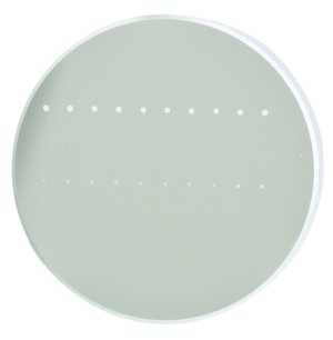
Figure 37A This photograph shows a protected aluminum-coated mirror after LIDT testing. In this particular test, it handled 0.43 J/cm2 (1064 nm, 10 ns pulse, 10 Hz, Ø1.000 mm) before damage.
Figure 37B Example Exposure Histogram used to Determine the LIDT of
| Table 37C Example Test Data | |||
|---|---|---|---|
| Fluence | # of Tested Locations | Locations with Damage | Locations Without Damage |
| 1.50 J/cm2 | 10 | 0 | 10 |
| 1.75 J/cm2 | 10 | 0 | 10 |
| 2.00 J/cm2 | 10 | 0 | 10 |
| 2.25 J/cm2 | 10 | 1 | 9 |
| 3.00 J/cm2 | 10 | 1 | 9 |
| 5.00 J/cm2 | 10 | 9 | 1 |
According to the test, the damage threshold of the mirror was 2.00 J/cm2 (532 nm, 10 ns pulse, 10 Hz, Ø0.803 mm). Please keep in mind that these tests are performed on clean optics, as dirt and contamination can significantly lower the damage threshold of a component. While the test results are only representative of one coating run, Thorlabs specifies damage threshold values that account for coating variances.
Continuous Wave and Long-Pulse Lasers
When an optic is damaged by a continuous wave (CW) laser, it is usually due to the melting of the surface as a result of absorbing the laser's energy or damage to the optical coating (antireflection) [1]. Pulsed lasers with pulse lengths longer than 1 µs can be treated as CW lasers for LIDT discussions.
When pulse lengths are between 1 ns and 1 µs, laser-induced damage can occur either because of absorption or a dielectric breakdown (therefore, a user must check both CW and pulsed LIDT). Absorption is either due to an intrinsic property of the optic or due to surface irregularities; thus LIDT values are only valid for optics meeting or exceeding the surface quality specifications given by a manufacturer. While many optics can handle high power CW lasers, cemented (e.g., achromatic doublets) or highly absorptive (e.g., ND filters) optics tend to have lower CW damage thresholds. These lower thresholds are due to absorption or scattering in the cement or metal coating.
Figure 37D LIDT in linear power density vs. pulse length and spot size. For long pulses to CW, linear power density becomes a constant with spot size. This graph was obtained from [1].
Figure 37E Intensity Distribution of Uniform and Gaussian Beam Profiles
Pulsed lasers with high pulse repetition frequencies (PRF) may behave similarly to CW beams. Unfortunately, this is highly dependent on factors such as absorption and thermal diffusivity, so there is no reliable method for determining when a high PRF laser will damage an optic due to thermal effects. For beams with a high PRF both the average and peak powers must be compared to the equivalent CW power. Additionally, for highly transparent materials, there is little to no drop in the LIDT with increasing PRF.
In order to use the specified CW damage threshold of an optic, it is necessary to know the following:
- Wavelength of your laser
- Beam diameter of your beam (1/e2)
- Approximate intensity profile of your beam (e.g., Gaussian)
- Linear power density of your beam (total power divided by 1/e2 beam diameter)
Thorlabs expresses LIDT for CW lasers as a linear power density measured in W/cm. In this regime, the LIDT given as a linear power density can be applied to any beam diameter; one does not need to compute an adjusted LIDT to adjust for changes in spot size, as demonstrated in Figure 37D. Average linear power density can be calculated using this equation.
This calculation assumes a uniform beam intensity profile. You must now consider hotspots in the beam or other non-uniform intensity profiles and roughly calculate a maximum power density. For reference, a Gaussian beam typically has a maximum power density that is twice that of the uniform beam (see Figure 37E).
Now compare the maximum power density to that which is specified as the LIDT for the optic. If the optic was tested at a wavelength other than your operating wavelength, the damage threshold must be scaled appropriately. A good rule of thumb is that the damage threshold has a linear relationship with wavelength such that as you move to shorter wavelengths, the damage threshold decreases (i.e., a LIDT of 10 W/cm at 1310 nm scales to 5 W/cm at 655 nm):
While this rule of thumb provides a general trend, it is not a quantitative analysis of LIDT vs wavelength. In CW applications, for instance, damage scales more strongly with absorption in the coating and substrate, which does not necessarily scale well with wavelength. While the above procedure provides a good rule of thumb for LIDT values, please contact Tech Support if your wavelength is different from the specified LIDT wavelength. If your power density is less than the adjusted LIDT of the optic, then the optic should work for your application.
Please note that we have a buffer built in between the specified damage thresholds online and the tests which we have done, which accommodates variation between batches. Upon request, we can provide individual test information and a testing certificate. The damage analysis will be carried out on a similar optic (customer's optic will not be damaged). Testing may result in additional costs or lead times. Contact Tech Support for more information.
Pulsed Lasers
As previously stated, pulsed lasers typically induce a different type of damage to the optic than CW lasers. Pulsed lasers often do not heat the optic enough to damage it; instead, pulsed lasers produce strong electric fields capable of inducing dielectric breakdown in the material. Unfortunately, it can be very difficult to compare the LIDT specification of an optic to your laser. There are multiple regimes in which a pulsed laser can damage an optic and this is based on the laser's pulse length. The highlighted columns in Table 37F outline the relevant pulse lengths for our specified LIDT values.
Pulses shorter than 10-9 s cannot be compared to our specified LIDT values with much reliability. In this ultra-short-pulse regime various mechanics, such as multiphoton-avalanche ionization, take over as the predominate damage mechanism [2]. In contrast, pulses between 10-7 s and 10-4 s may cause damage to an optic either because of dielectric breakdown or thermal effects. This means that both CW and pulsed damage thresholds must be compared to the laser beam to determine whether the optic is suitable for your application.
| Table 37F Laser Induced Damage Regimes | ||||
|---|---|---|---|---|
| Pulse Duration | t < 10-9 s | 10-9 < t < 10-7 s | 10-7 < t < 10-4 s | t > 10-4 s |
| Damage Mechanism | Avalanche Ionization | Dielectric Breakdown | Dielectric Breakdown or Thermal | Thermal |
| Relevant Damage Specification | No Comparison (See Above) | Pulsed | Pulsed and CW | CW |
When comparing an LIDT specified for a pulsed laser to your laser, it is essential to know the following:
Figure 37G LIDT in energy density vs. pulse length and spot size. For short pulses, energy density becomes a constant with spot size. This graph was obtained from [1].
- Wavelength of your laser
- Energy density of your beam (total energy divided by 1/e2 area)
- Pulse length of your laser
- Pulse repetition frequency (prf) of your laser
- Beam diameter of your laser (1/e2 )
- Approximate intensity profile of your beam (e.g., Gaussian)
The energy density of your beam should be calculated in terms of J/cm2. Figure 37G shows why expressing the LIDT as an energy density provides the best metric for short pulse sources. In this regime, the LIDT given as an energy density can be applied to any beam diameter; one does not need to compute an adjusted LIDT to adjust for changes in spot size. This calculation assumes a uniform beam intensity profile. You must now adjust this energy density to account for hotspots or other nonuniform intensity profiles and roughly calculate a maximum energy density. For reference a Gaussian beam typically has a maximum energy density that is twice that of the 1/e2 beam.
Now compare the maximum energy density to that which is specified as the LIDT for the optic. If the optic was tested at a wavelength other than your operating wavelength, the damage threshold must be scaled appropriately [3]. A good rule of thumb is that the damage threshold has an inverse square root relationship with wavelength such that as you move to shorter wavelengths, the damage threshold decreases (i.e., a LIDT of 1 J/cm2 at 1064 nm scales to 0.7 J/cm2 at 532 nm):
You now have a wavelength-adjusted energy density, which you will use in the following step.
Beam diameter is also important to know when comparing damage thresholds. While the LIDT, when expressed in units of J/cm², scales independently of spot size; large beam sizes are more likely to illuminate a larger number of defects which can lead to greater variances in the LIDT [4]. For data presented here, a <1 mm beam size was used to measure the LIDT. For beams sizes greater than 5 mm, the LIDT (J/cm2) will not scale independently of beam diameter due to the larger size beam exposing more defects.
The pulse length must now be compensated for. The longer the pulse duration, the more energy the optic can handle. For pulse widths between 1 - 100 ns, an approximation is as follows:
Use this formula to calculate the Adjusted LIDT for an optic based on your pulse length. If your maximum energy density is less than this adjusted LIDT maximum energy density, then the optic should be suitable for your application. Keep in mind that this calculation is only used for pulses between 10-9 s and 10-7 s. For pulses between 10-7 s and 10-4 s, the CW LIDT must also be checked before deeming the optic appropriate for your application.
Please note that we have a buffer built in between the specified damage thresholds online and the tests which we have done, which accommodates variation between batches. Upon request, we can provide individual test information and a testing certificate. Contact Tech Support for more information.
[1] R. M. Wood, Optics and Laser Tech. 29, 517 (1998).
[2] Roger M. Wood, Laser-Induced Damage of Optical Materials (Institute of Physics Publishing, Philadelphia, PA, 2003).
[3] C. W. Carr et al., Phys. Rev. Lett. 91, 127402 (2003).
[4] N. Bloembergen, Appl. Opt. 12, 661 (1973).

In order to illustrate the process of determining whether a given laser system will damage an optic, a number of example calculations of laser induced damage threshold are given below. For assistance with performing similar calculations, we provide a spreadsheet calculator that can be downloaded by clicking the LIDT Calculator button. To use the calculator, enter the specified LIDT value of the optic under consideration and the relevant parameters of your laser system in the green boxes. The spreadsheet will then calculate a linear power density for CW and pulsed systems, as well as an energy density value for pulsed systems. These values are used to calculate adjusted, scaled LIDT values for the optics based on accepted scaling laws. This calculator assumes a Gaussian beam profile, so a correction factor must be introduced for other beam shapes (uniform, etc.). The LIDT scaling laws are determined from empirical relationships; their accuracy is not guaranteed. Remember that absorption by optics or coatings can significantly reduce LIDT in some spectral regions. These LIDT values are not valid for ultrashort pulses less than one nanosecond in duration.
Figure 71A A Gaussian beam profile has about twice the maximum intensity of a uniform beam profile.
CW Laser Example
Suppose that a CW laser system at 1319 nm produces a 0.5 W Gaussian beam that has a 1/e2 diameter of 10 mm. A naive calculation of the average linear power density of this beam would yield a value of 0.5 W/cm, given by the total power divided by the beam diameter:
However, the maximum power density of a Gaussian beam is about twice the maximum power density of a uniform beam, as shown in Figure 71A. Therefore, a more accurate determination of the maximum linear power density of the system is 1 W/cm.
An AC127-030-C achromatic doublet lens has a specified CW LIDT of 350 W/cm, as tested at 1550 nm. CW damage threshold values typically scale directly with the wavelength of the laser source, so this yields an adjusted LIDT value:
The adjusted LIDT value of 350 W/cm x (1319 nm / 1550 nm) = 298 W/cm is significantly higher than the calculated maximum linear power density of the laser system, so it would be safe to use this doublet lens for this application.
Pulsed Nanosecond Laser Example: Scaling for Different Pulse Durations
Suppose that a pulsed Nd:YAG laser system is frequency tripled to produce a 10 Hz output, consisting of 2 ns output pulses at 355 nm, each with 1 J of energy, in a Gaussian beam with a 1.9 cm beam diameter (1/e2). The average energy density of each pulse is found by dividing the pulse energy by the beam area:
As described above, the maximum energy density of a Gaussian beam is about twice the average energy density. So, the maximum energy density of this beam is ~0.7 J/cm2.
The energy density of the beam can be compared to the LIDT values of 1 J/cm2 and 3.5 J/cm2 for a BB1-E01 broadband dielectric mirror and an NB1-K08 Nd:YAG laser line mirror, respectively. Both of these LIDT values, while measured at 355 nm, were determined with a 10 ns pulsed laser at 10 Hz. Therefore, an adjustment must be applied for the shorter pulse duration of the system under consideration. As described on the previous tab, LIDT values in the nanosecond pulse regime scale with the square root of the laser pulse duration:
This adjustment factor results in LIDT values of 0.45 J/cm2 for the BB1-E01 broadband mirror and 1.6 J/cm2 for the Nd:YAG laser line mirror, which are to be compared with the 0.7 J/cm2 maximum energy density of the beam. While the broadband mirror would likely be damaged by the laser, the more specialized laser line mirror is appropriate for use with this system.
Pulsed Nanosecond Laser Example: Scaling for Different Wavelengths
Suppose that a pulsed laser system emits 10 ns pulses at 2.5 Hz, each with 100 mJ of energy at 1064 nm in a 16 mm diameter beam (1/e2) that must be attenuated with a neutral density filter. For a Gaussian output, these specifications result in a maximum energy density of 0.1 J/cm2. The damage threshold of an NDUV10A Ø25 mm, OD 1.0, reflective neutral density filter is 0.05 J/cm2 for 10 ns pulses at 355 nm, while the damage threshold of the similar NE10A absorptive filter is 10 J/cm2 for 10 ns pulses at 532 nm. As described on the previous tab, the LIDT value of an optic scales with the square root of the wavelength in the nanosecond pulse regime:
This scaling gives adjusted LIDT values of 0.08 J/cm2 for the reflective filter and 14 J/cm2 for the absorptive filter. In this case, the absorptive filter is the best choice in order to avoid optical damage.
Pulsed Microsecond Laser Example
Consider a laser system that produces 1 µs pulses, each containing 150 µJ of energy at a repetition rate of 50 kHz, resulting in a relatively high duty cycle of 5%. This system falls somewhere between the regimes of CW and pulsed laser induced damage, and could potentially damage an optic by mechanisms associated with either regime. As a result, both CW and pulsed LIDT values must be compared to the properties of the laser system to ensure safe operation.
If this relatively long-pulse laser emits a Gaussian 12.7 mm diameter beam (1/e2) at 980 nm, then the resulting output has a linear power density of 5.9 W/cm and an energy density of 1.2 x 10⁻⁴ J/cm2 per pulse. This can be compared to the LIDT values for a WPQ10E-980 polymer zero-order quarter-wave plate, which are 5 W/cm for CW radiation at 810 nm and 5 J/cm2 for a 10 ns pulse at 810 nm. As before, the CW LIDT of the optic scales linearly with the laser wavelength, resulting in an adjusted CW value of 6 W/cm at 980 nm. On the other hand, the pulsed LIDT scales with the square root of the laser wavelength and the square root of the pulse duration, resulting in an adjusted value of 55 J/cm2 for a 1 µs pulse at 980 nm. The pulsed LIDT of the optic is significantly greater than the energy density of the laser pulse, so individual pulses will not damage the wave plate. However, the large average linear power density of the laser system may cause thermal damage to the optic, much like a high-power CW beam.
KLC101 Software
Version 1.0.0
GUI Interface for controlling the KLC101 Liquid Crystal Contoller via a PC. To download, click the Software button.
LCC25D Software
Version 1.0.0
GUI Interface for controlling the LCC25D Liquid Crystal Controller via a PC. To download, click the Software button.
LCC25 Software
Version 4.0.1
GUI Interface for controlling the LCC25 Liquid Crystal Controller via a PC. To download, click the Software button.
| Posted Comments: | |
| No Comments Posted |

 Zoom
Zoom
Click to Enlarge
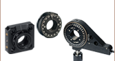
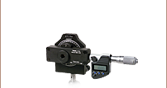
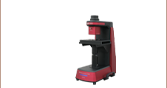
Figure G1.1 The polarization rotators can be mounted in an RSP1(/M) rotation mount for ease of alignment.
- 532 nm or 633 nm Operating Wavelength
- Ø10 mm Clear Aperture
- 1" Outer Diameter
Thorlabs' Ø10 mm clear aperture, LC polarization rotators are available with operating wavelengths of 532 nm or 633 nm. Acceptable input polarization axes are indicated by engraved lines on the front of the rotator housing. Each rotator has an approximately 930 mm long BNC cable for connecting the device to a driver, such as the LCC25, LCC25D, or KLC101 controllers available below. These retarders have an outer diameter of 1", making them compatible with any of our Ø1" optic mounts for 9.4 mm thick optics, such as the RSP1(/M) rotation mount for post mounting or the CRM1PT(/M) rotation mount for 30 mm cage system compatibility.

 Zoom
Zoom
- 0 to ±25 VAC Square-Wave Output Voltage
- LCC25: 2000 ± 5 Hz
- LCC25D and KLC101: Adjustable from 500 Hz to 10 kHz
- Internal and External Options for Modulating the Output Square-Wave Amplitude
- Edit Settings Using Device Panel or Control from a PC
The LCC25, LCC25D, and KLC101 Liquid Crystal (LC) Controllers are each designed to operate Thorlabs' liquid crystal cells, rotators, and retarders (except for the LCC2415-VIS, which has an integrated controller). Each controller supplies a a square-wave AC voltage output with an amplitude that can be adjusted from 0 VRMS to ±25 VRMS. To increase the lifetime of liquid crystal devices, these controllers will automatically detect and correct any DC offset to within ±10 mV in real time.
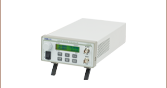
LCC25 Benchtop Controller
The LCC25 LC Controller produces a 2000 Hz square-wave AC voltage output with an amplitude that can be set using the front panel controls, an external 0 - 5 VDC TTL input, or via the USB interface. When the LCC25 controller is operated in the constant voltage mode, the output of the controller will be a 2000 Hz square wave with a user-set amplitude. Alternatively, in Modulation mode, the amplitude of the 2000 Hz square wave output will switch between user-defined values V1 and V2 at a frequency that can be set internally (0.5 Hz to 150 Hz, see Figure 1.2, bottom) or triggered externally with 0 to 5 V TTL input (0.5 Hz to 500 Hz). The modulated mode can also be used to measure the response time of the connected LC retarder. The LCC25 controller's software package also allows the user to define a voltage sequence by specifying a starting voltage, ending voltage, voltage step size, and dwell time.
LCC25D Benchtop Controller
The LCC25D LC Controller supplies a square-wave AC output voltage with a user-set amplitude and frequency from 500 Hz to 10 kHz that can be set using its front panel controls, an external 0 - 5 VDC TTL input, or via the USB or an additional ethernet interface. When operated in "V1" or "V2" mode, the output signal will be an AC square wave with a constant RMS voltage amplitude. In "Switch" mode, the output signal will be an AC square wave at an RMS voltage level switching between the values currently set for Voltage 1 and Voltage 2 at the frequency set internally (0.5 Hz to 150 Hz) or triggered externally with 0 to 5 V TTL input (0.1 Hz to 150 Hz). "Switch" mode can also be used to measure the response time of the connected LC retarder.
The LCC25D controller features an additional fast-switching function that allows setting two additional voltages for a total of four voltages that the output can switch between in a cycle. The LCC25D controller also has a heating function with a max set point of 50 °C for temperature-stabilized LC devices, with 0.1 °C resolution.
The LCC25 and LCC25D controllers' software packages also allow the user to define a voltage sequence by specifying a starting voltage, ending voltage, voltage step size, and dwell time. Please visit the benchtop LC controllers page for more information on these controllers.
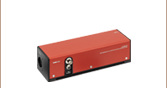
KLC101 K-Cube® Controller
The KLC101 K-Cube® LC Controller is a part of Thorlabs' growing line of high-end, compact controllers. It supplies a square-wave AC output voltage with a user-set frequency from 500 Hz to 10 kHz and features a small 60.0 mm x 60.0 mm footprint. The controller top panel, software, and trigger ports allow the user to create customized output voltage and frequency sequences. The voltage can be set to switch between two preset values at rates from 0.1 and 150 Hz using the top panel controls or software. When in this mode, one of the trigger ports will output a 5 V logic signal indicating when the voltage is switched. Alternatively, a trigger port can be used as an input for the 5 V logic signal to switch between the preset voltages. The software also enables Sequence and Sweep Modes for setting custom output sequences.
Note that the KLC101 controller does not ship with a power supply. For applications requiring a single K-Cube, the TPS002 power supply (sold below) can be used. We also offer USB controller hubs for use with multiple K-Cubes.
See the full KLC101 controller web presentation for more information on the features of this controller and its power supply options.
| Item # | Adjustable Output Voltage |
Voltage Resolution |
Adjustable Output Frequencya |
Internal Modulationa |
External Modulation |
Slew Rate |
DC Offset |
Warm Up Time |
Output Current (Max) |
External Input Voltage (Max) |
Temperature Setting Range |
|---|---|---|---|---|---|---|---|---|---|---|---|
| LCC25 | 0 to ±25 V RMS | 1.0 mV | 2,000 ± 5 Hz | 0.5 to 150 Hz | 0.5 to 500 Hz | 10 V/µs | ±10 mV | 30 Minutes | 15 mA | 5 VDC | N/A |
| LCC25D | 500 Hz to 10 kHz | 0.1 to 150 Hza | 50 mA | 10 to 50 °C, Resolution 0.1 °C |
|||||||
| KLC101 | 0.1 to 150 Hz | 150 Hz (Max) | N/A |