 Products Home / Optical Systems / Objective Lenses, Scan Lenses, and Tube Lenses / Microscope Objectives for Life Sciences, Dry
Microscope Objectives for Life Sciences, Dry
- Infinity-Corrected Dry Microscope Objectives
- Axial Color Correction Options Across the Visible and NIR Spectrum
- Designed for Widefield Fluorescence or Multiphoton Imaging Applications
- 1X, 2X, 4X, 10X, or 15X Magnification
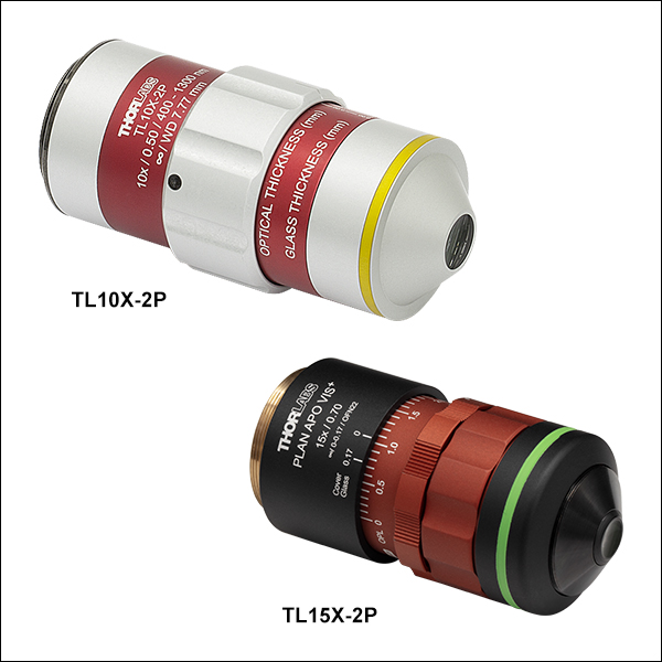
TL10X-2P
10X Super Apochromat Objective for Two-Photon Microscopy
TL2X-SAP
2X Super Apochromat Objective
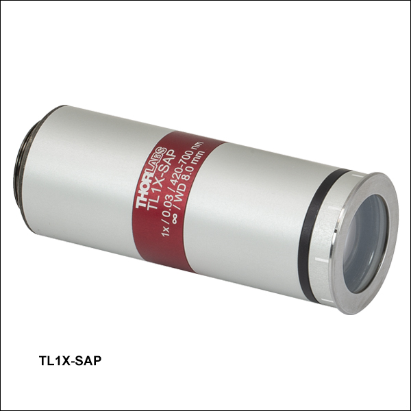
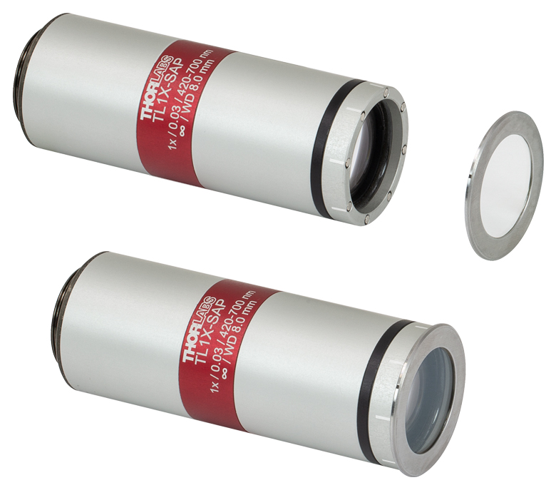
TL1X-SAP
1X Super Apochromat Objective
TL15X-2P
15X Plan Apochromat VIS+ Objective for Two-Photon Microscopy


Please Wait

| Objective Lens Selection Guide |
|---|
| Objectives |
| Microscopy Objectives for Life Sciences, Dry Microscopy Objectives, Dry Microscopy Objectives, Oil Immersion Physiology Objectives, Water Dipping or Immersion Phase Contrast Objectives Long Working Distance Objectives Reflective Microscopy Objectives UV Microscopy Objectives VIS and NIR Focusing Objectives |
| Scan Lenses and Tube Lenses |
| Scan Lenses Infinity-Corrected Tube Lens |
| Webpage Features | |
|---|---|
 |
Zemax blackbox files for the objectives on this page can be accessed by clicking this icon below. |

Did You Know?
Multiple optical elements, including the microscope objective, tube lens, and eyepieces, together define the magnification of a system. See the Magnification & FOV tab to learn more.
Click for Details
Thorlabs maintains the labeling convention shown above for all of its super apochromatic microscope objectives. (See the Objective Tutorial tab for more information about microscope objective types.)
Click for Details
Thorlabs maintains the labeling convention shown above for its TL15X-2P objective. (See the Objective Tutorial tab for more information about microscope objective types.)
Features
- Infinity-Corrected Super Apochromatic and Enhanced Visible Design
- Antireflection (AR) Coatings:
- 1X Objective: 420 nm - 700 nm
- 2X and 4X Objectives: 350 nm - 700 nm
- 10X and 15X Objectives: 400 nm - 1300 nm
- Numerical Aperture (NA) Up to 0.70
- Ideal for Brightfield, Fluorescence, Multiphoton, or Confocal Imaging Applications
- Magnifications Specified for Use with a 200 mm Tube Lens
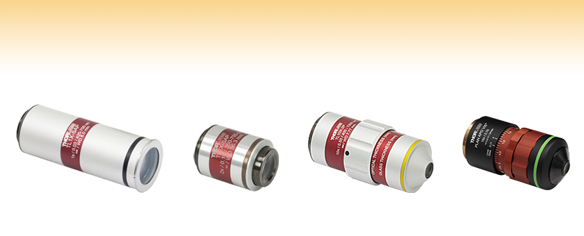
Thorlabs' apochromatic microscope objectives for life sciences provide axial color correction across the visible range and a flat field of focus in a variety of imaging modalities without introducing vignetting. These objectives are designed for use with a tube lens focal length of 200 mm and have optical elements that are AR-coated for improved transmission. Our 1X telecentric objective is ideal for machine vision applications (see Telecentric Tutorial tab), while our 2X and 4X objectives have higher numerical apertures (NA) of 0.10 and 0.20, respectively, making them ideal for widefield imaging. Lastly, our 10X and 15X objectives are designed for two-photon imaging. These objectives have 7.77 mm and 2.60 mm working distances respectively and feature a correction collar and optical thickness scale, allowing the objectives' focus to be adjusted for a variety of media that may be present between the objective and the sample, such as aqueous solutions and cover glasses (see the Correction Collar tab for details). Note that these objectives are not suitable for water-dipping, water-immersion, or oil-immersion techniques.
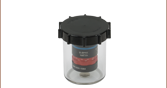
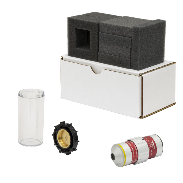
Every objective housing is engraved with the Item #, magnification, NA, and wavelength range. Each objective is shipped in an objective case comprised of a lid and container. The threading for each objective is given below; to use the objectives with a different thread standard, please see our microscope objective thread adapters.
Mounting the objectives on this page together or in combination with other objectives may require parfocal length extenders, which allow users to match parfocal lengths and switch between objectives of different magnifications mounted in a turret or nosepiece without significant refocusing.
| Item # | TL1X-SAPa | TL2X-SAP | TL4X-SAP | TL10X-2P | TL15X-2P |
|---|---|---|---|---|---|
| Specifications | |||||
| Magnificationb | 1X | 2X | 4X | 10X | 15X |
| Numerical Aperture (NA) | 0.03 | 0.10 | 0.20 | 0.50 | 0.70 |
| AR Coating Range | 420 - 700 nm | 350 - 700 nm | 400 - 1300 nm | ||
| AR Coating Reflectance Per Surface |
Ravg < 0.5% @ 0° AOI | Rabs < 3% (400 - 450 nm) Rabs < 2% (450 - 1300 nm) @ 0° - 25° AOI |
|||
| Total Transmission (Click to Enlarge) |
Raw Data |
Raw Data |
Raw Data |
Raw Data |
Raw Data |
| Axial Colorc | Diffraction Limited over 440 - 700 nm | Diffraction Limited over |
|||
| Field of View | Ø22 mm | Ø11 mm | Ø5.5 mm | Ø2.2 mm | Ø1.5 mm |
| Working Distanced | 8.0 mm | 56.3 mm | 17.0 mm | 7.77 mm | 2.6 mme |
| Effective Focal Length (EFL) | 200 mm | 100 mm | 50 mm | 20 mm | 13.3 mm |
| Entrance Pupil Diameter | 12.0 mmf | 20.0 mmf | 20.0 mmf | 20.0 mmg | 18.6 mmg |
| Resolutionh | 11.2 µm | 3.4 µm | 1.7 µm | 0.7 µm | 0.5 µm |
| Parfocal Lengthd | 95.0 mm | 95.0 mm | 60.0 mmi | 95.0 mm | 75.0 mm |
| Diameterd | 32.6 mm (Without Wave Plate) |
30.5 mm | 43.2 mm | 38.1 mm | |
| 34.5 mm (With Wave Plate) |
|||||
| Lengthd | 85.5 mm (Without Wave Plate) |
43.5 mm | 46.4 mm | 90.4 mm | 76.9 mm |
| 90.6 mm (With Wave Plate) |
|||||
| Housing Threads | M25 x 0.75 | M32 x 0.75 | |||
| Thread Depth | 3.8 mm | 3.2 mm | 3.6 mm | 3.2 mm | 4.5 mm |
| Field Numberj | 22 | ||||
| Design Tube Lens Focal Lengthk | 200 mm | ||||
| Cover Glass Thickness | 0 - 5.0 mm | 0 - 5.0 mm | 0 - 5.0 mm | 0 - 2.6 mm | 0 - 2.8 mm |
| Recommended Microscopy Techniques | |||||
| Confocal | |||||
| Two-Photon | - | - | - | ||
| Brightfield | |||||
| Darkfield | |||||
| Dodt | |||||
| DIC | - | - | |||
| Fluorescence | |||||
Objective Performance Data
Various tests were carried out to demonstrate the specified performance of each of our objectives. Click the links below for more information about a specific objective.
1X Objective Performance Graphs
Click here for raw data for all plots.
Click to Enlarge
Transmission of the TL1X-SAP Objective. The blue shaded region denotes the wavelength range of the AR coating.
Click to Enlarge
Axial color describes the shift in the image plane across the operating wavelength range of the 1X super apochromatic microscope objective. The pink shaded region denotes diffraction-limited performance.
Click to Enlarge
The Strehl Ratio is a quantitative measurement of optical image formation quality. The Strehl Ratio for the TL1X-SAP over its field of view is shown in the graph above.
Click to Enlarge
This graph shows the Strehl Ratio of the TL1X-SAP over the objective's full operating wavelength range.
2X Objective Performance Graphs
Click here for raw data for all plots.
Click to Enlarge
Transmission of the TL2X-SAP Objective. The blue shaded region denotes the wavelength range of the AR coating.
Click to Enlarge
Axial color describes the shift in the image plane across the operating wavelength range of the 2X super apochromatic microscope objective. The pink shaded region denotes diffraction-limited performance.
Click to Enlarge
The Strehl Ratio is a quantitative measurement of optical image formation quality. The Strehl Ratio for the TL2X-SAP over its field of view is shown in the graph above.
Click to Enlarge
This graph shows the Strehl Ratio of the TL2X-SAP over the objective's full operating wavelength range.
4X Objective Performance Graphs
Click here for raw data for all plots.
Click to Enlarge
Transmission of the TL4X-SAP Objective. The blue shaded region denotes the wavelength range of the AR coating.
Click to Enlarge
Axial color describes the shift in the image plane across the operating wavelength range of the 4X super apochromatic microscope objective. The pink shaded region denotes diffraction-limited performance.

Click to Enlarge
The Strehl Ratio is a quantitative measurement of optical image formation quality. The Strehl Ratio for the TL4X-SAP over its field of view is shown in the graph above.
Click to Enlarge
This graph shows the Strehl Ratio of the TL4X-SAP over the objective's full operating wavelength range.
10X Objective Performance Graphs
Click here for raw data for all plots.
Click to Enlarge
Transmission of the TL10X-2P Objective. The blue shaded region denotes the wavelength range of the AR coating.
Click to Enlarge
Axial color describes the shift in the image plane across the operating wavelength range of the 10X super apochromatic microscope objective. The pink shaded region denotes diffraction-limited performance. Diffraction-limited performance can be shifted to the NIR with refocusing.
Click to Enlarge
The Strehl Ratio is a quantitative measurement of optical image formation quality. The Strehl Ratio for the TL10X-SAP over its field of view is shown in the graph above.
Click to Enlarge
This graph shows the Strehl Ratio of the TL10X-2P over the objective's visible performance band.

Click to Enlarge
The Group Delay Dispersion (GDD) represents how the duration of an ultrafast laser pulse will increase through an optical path length. The simulated GDD for the TL10X-2P objective is shown in the graph above.
15X Objective Performance Graphs
Click here for raw data for all plots.
Click to Enlarge
Transmission of the TL15X-2P Objective. The blue shaded region denotes the wavelength range of the AR coating.
Click to Enlarge
Axial color describes the shift in the image plane across the operating wavelength range of the 15X apochromatic improved visible microscope objective. The pink shaded region denotes diffraction-limited performance. Diffraction-limited performance can be shifted to the NIR with refocusing.
Click to Enlarge
The Strehl Ratio is a quantitative measurement of optical image formation quality. The Strehl Ratio for the TL15X-2P over its field of view is shown in the graph above.

Click to Enlarge
This graph shows the Strehl Ratio of the TL15X-2P over the objective's visible performance band.
Click to Enlarge
The Group Delay Dispersion (GDD) represents how the duration of an ultrafast laser pulse will increase through an optical path length. The simulated GDD for the TL15X-2P objective is shown in the graph above.
| Table 89A Chromatic Aberration Correction per ISO Standard 19012-2 | ||
|---|---|---|
| Objective Class | Common Abbreviations | Axial Focal Shift Tolerancesa |
| Achromat | ACH, ACHRO, ACHROMAT | |δC' - δF'| ≤ 2 x δob |
| Semiapochromat (or Fluorite) |
SEMIAPO, FL, FLU | |δC' - δF'| ≤ 2 x δob |δF' - δe| ≤ 2.5 x δob |δC' - δe| ≤ 2.5 x δob |
| Apochromat | APO | |δC' - δF'| ≤ 2 x δob |δF' - δe| ≤ δob |δC' - δe| ≤ δob |
| Super Apochromat | SAPO | See Footnote b |
| Improved Visible Apochromat | VIS+ | See Footnotes b and c |
Parts of a Microscope Objective
Click on each label for more details.
Figure 89C This microscope objective serves only as an example. The features noted above with an asterisk may not be present on all objectives; they may be added, relocated, or removed from objectives based on the part's needs and intended application space.
Objective Tutorial
This tutorial describes features and markings of objectives and what they tell users about an objective's performance.
Objective Class and Aberration Correction
Objectives are commonly divided by their class. An objective's class creates a shorthand for users to know how the objective is corrected for imaging aberrations. There are two types of aberration corrections that are specified by objective class: field curvature and chromatic aberration.
Field curvature (or Petzval curvature) describes the case where an objective's plane of focus is a curved spherical surface. This aberration makes widefield imaging or laser scanning difficult, as the corners of an image will fall out of focus when focusing on the center. If an objective's class begins with "Plan", it will be corrected to have a flat plane of focus.
Images can also exhibit chromatic aberrations, where colors originating from one point are not focused to a single point. To strike a balance between an objective's performance and the complexity of its design, some objectives are corrected for these aberrations at a finite number of target wavelengths.
Five objective classes are shown in Table 89A; only three common objective classes are defined under the International Organization for Standards ISO 19012-2: Microscopes -- Designation of Microscope Objectives -- Chromatic Correction. Due to the need for better performance, we have added two additional classes that are not defined in the ISO classes.
Immersion Methods
Click on each image for more details.
Figure 89B Objectives can be divided by what medium they are designed to image through. Dry objectives are used in air; whereas dipping and immersion objectives are designed to operate with a fluid between the objective and the front element of the sample.
| Glossary of Terms | |
|---|---|
| Back Focal Length and Infinity Correction | The back focal length defines the location of the intermediate image plane. Most modern objectives will have this plane at infinity, known as infinity correction, and will signify this with an infinity symbol (∞). Infinity-corrected objectives are designed to be used with a tube lens between the objective and eyepiece. Along with increasing intercompatibility between microscope systems, having this infinity-corrected space between the objective and tube lens allows for additional modules (like beamsplitters, filters, or parfocal length extenders) to be placed in the beam path. Note that older objectives and some specialty objectives may have been designed with finite back focal lengths. In their inception, finite back focal length objectives were meant to interface directly with the objective's eyepiece. |
| Entrance Pupil Diameter (EP) | The entrance pupil diameter (EP), sometimes referred to as the entrance aperture diameter, corresponds to the appropriate beam diameter one should use to allow the objective to function properly. EP = 2 × NA × Effective Focal Length |
| Field Number (FN) and Field of View (FOV) |
The field number corresponds to the diameter of the field of view in object space (in millimeters) multiplied by the objective's magnification. Field Number = Field of View Diameter × Magnification |
| Magnification (M) | The magnification (M) of an objective is the lens tube focal length (L) divided by the objective's effective focal length (F). Effective focal length is sometimes abbreviated EFL: M = L / EFL . The total magnification of the system is the magnification of the objective multiplied by the magnification of the eyepiece or camera tube. The specified magnification on the microscope objective housing is accurate as long as the objective is used with a compatible tube lens focal length. Objectives will have a colored ring around their body to signify their magnification. This is fairly consistent across manufacturers; see the Parts of a Microscope Objective section for more details. |
| Numerical Aperture (NA) | Numerical aperture, a measure of the acceptance angle of an objective, is a dimensionless quantity. It is commonly expressed as: NA = ni × sinθa where θa is the maximum 1/2 acceptance angle of the objective, and ni is the index of refraction of the immersion medium. This medium is typically air, but may also be water, oil, or other substances. |
| Working Distance (WD) |
The working distance, often abbreviated WD, is the distance between the front element of the objective and the top of the specimen (in the case of objectives that are intended to be used without a cover glass) or top of the cover glass, depending on the design of the objective. The cover glass thickness specification engraved on the objective designates whether a cover glass should be used. |
A cover glass, or coverslip, is a small, thin sheet of glass that can be placed on a wet sample to create a flat surface to image across.
The most common, a standard #1.5 cover glass, is designed to be 0.17 mm thick. Due to variance in the manufacturing process the actual thickness may be different. The correction collar present on select objectives is used to compensate for cover glasses of different thickness by adjusting the relative position of internal optical elements. Note that many objectives do not have a variable cover glass correction, in which case the objectives have no correction collar. For example, an objective could be designed for use with only a #1.5 cover glass. This collar may also be located near the bottom of the objective, instead of the top as shown in the diagram.
Click to Enlarge
The graph above shows the magnitude of spherical aberration versus the thickness of the coverslip used for 632.8 nm light. For the typical coverslip thickness of 0.17 mm, the spherical aberration caused by the coverslip does not exceed the diffraction-limited aberration for objectives with NA up to 0.40.
Click to Enlarge
This graph shows the effect of a cover slip on image quality at 632.8 nm for a #1.5 cover glass (0.17 mm thickness) with a refractive index of 1.51.
Click for Details
Thickness and Light Cone Dramatized for Readability
Correction Collar and Cover Glass Correction
A cover glass is often placed onto an aqueous specimen to create a flat top on a volume to image. While this makes focusing on a sample easier, the presence of the glass can introduce spherical aberrations in the final image. The graph to the right shows the magnitude of spherical aberration versus the thickness of the cover glass used, for 632.8 nm light. For the typical cover glass thickness of 0.17 mm, the spherical aberration caused by the cover glass does not exceed the diffraction-limited aberration for objectives with NA up to 0.40.
Our TL10X-2P and TL15X-2P microscope objectives are equipped with a correction collar, which compensates for cover glasses of different thickness by adjusting the relative position of internal optical elements, reducing the impact of spherical aberration to help achieve diffraction-limited performance. Their correction collars feature two scales: one for the thickness of a cover glass with a refractive index of 1.51 and a second that corresponds to the optical thickness of the material between the objective and the focal plane (ignoring air). The latter is useful for cases where the region of interest is suspended in a solution. Values on both scales are given in units of millimeters.
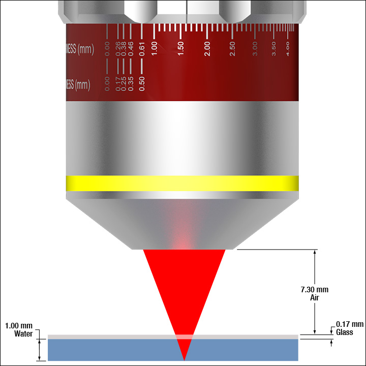
To find the optical thickness of all non-air elements between your objective and your sample, multiply the thickness of an element in millimeters by its refractive index, and find the sum of all such products. For example, suppose that the TL10X-2P objective is focusing through 7.30 mm of air, a 0.17 mm cover slip, and 1.00 mm of saline solution, as illustrated in the image to the lower right. To find the appropriate correction collar setting, multiply each thickness, t, by each material's refractive index, n, ignoring air:
Optical Thickness Collar Setting = ∑txnx
t1n1 + t2n2 = 0.17 mm × 1.51 + 1.00 mm × 1.33 = 1.59 mm
| Examples of Optical Thickness Calculationsa | ||
|---|---|---|
| Glass Thickness (n = 1.51) |
Water Thickness (n = 1.33) |
Optical Thickness Collar Setting |
| 0.00 mm | 0.00 mm | 0.00 mm |
| 0.50 mm | 0.00 mm | 0.76 mm |
| 0.17 mm | 1.00 mm | 1.59 mm |
| 0.17 mm | 3.00 mm | 4.25 mm |
Our other super apochromatic objectives do not have a correction collar. While they are designed for use with a standard 0.17 mm thick cover glass, their NAs are low enough (0.2 or less) that any cover glass thickness between 0 and 0.5 mm can be used with little impact on image quality.
Telecentric Lenses
Telecentric lenses are designed to have a constant magnification regardless of the object's distance or location in the field of view. This attribute is ideal for many machine vision measurement applications, as measurements of an object's dimensions will be independent of where it is located.
Types of Telecentric Lenses
In order to achieve a telecentric lens design, all of the chief rays (rays from an off-axis point that pass through the center of the aperture stop) have to be parallel to the optical axis in either image space or object space, or both.
For an object space telecentric lens, the chief rays will be parallel to the optical axis on the object's side of the lens (object space). This is accomplished by setting the aperture stop at the front focal plane of the lens, which results in an entrance pupil at infinity. Since chief rays are directed towards the center of the entrance pupil, the chief rays on the object side of the lens will be parallel to the optical axis. An example of an object space telecentric lens is shown in Figure 119A.
For an image space telecentric lens, the chief rays will be parallel to the optical axis on the image's side of the lens (image space). This is accomplished by setting the aperture stop at the back focal plane of the lens, which results in an exit pupil at infinity. Since the chief rays must pass through the center of the exit pupil, the chief rays on the image side of the lens must be parallel to the optical axis. An example of an image space telecentric lens is shown in Figure 119B.
Click to Enlarge
Figure 119A A ray trace through an idealized object space telecentric lens system. Note that the chief rays (the center ray of each color) are parallel to the optical axis in object space, but in image space, the chief rays form an angle with the optical axis.
Click to Enlarge
Figure 119B A ray trace through an idealized image space telecentric lens system. Note that the chief rays (the center ray of each color) are parallel to the optical axis in image space, but in object space, the chief rays form an angle with the optical axis.
For a double telecentric, or bi-telecentric, lens, the front and back focal planes are made to overlap so that the aperture stop is located where both the entrance and exit pupils are at infinity. In a bi-telecentric lens, neither the image or object location will affect the magnification. Thorlabs' telecentric lenses are all bi-telecentric designs. Figure 119C shows an example ray trace through a bi-telecentric lens and illustrates how the chief rays pass through the system.
Click to Enlarge
Figure 119C A ray trace through an idealized bi-telecentric lens system. Note that the chief rays (the center ray of each color) are parallel to the optical axis in both image and object space, which means that the magnification will remain constant regardless of object distance.
Conventional Lenses
In conventional lenses, the entrance and exit pupils are not located at infinity, so the chief rays will not be parallel to the optical axis. In this case, the magnification of the object depends on its distance from the lens and its position in the field of view. Figure 119D shows an example ray trace through a conventional camera lens; notice how the chief rays are angled with respect to the optical axis in both image and object space. Note that both Figures 119C and 119D feature the same lens design; only the aperture stop location was varied to shift the bi-telecentric system to a non-telecentric one.
Click to Enlarge
Figure 119D A ray trace through an idealized conventional camera lens system. Note that the chief rays (the center ray of each color) are not parallel to the optical axis in both image and object space, which means that the magnification will vary with object distance.
Example Images
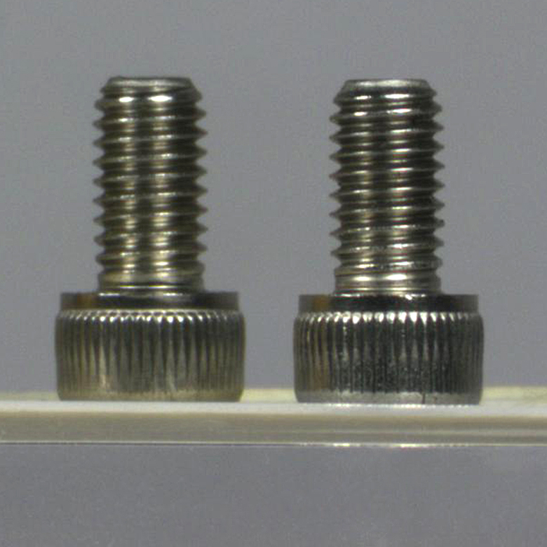
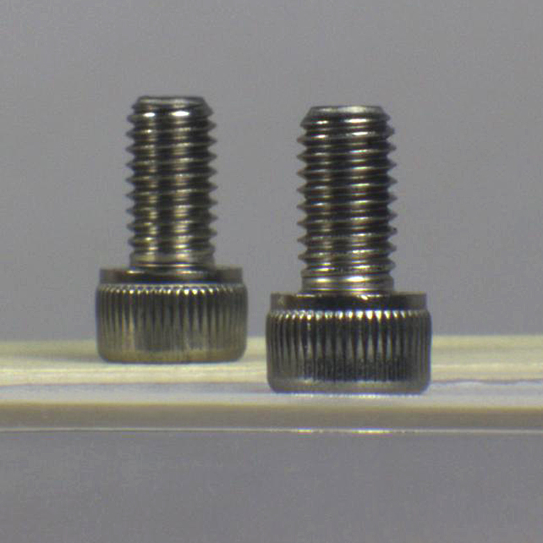
Figures 119E and 119F show photographs taken with a bi-telecentric lens and a standard camera lens, respectively. With the telecentric imaging system, the height of the two screws appears to be the same, even though the object planes are separated by approximately 45 mm along the optical axis. With the conventional imaging system, the two screws appear to be different heights, which could result in inaccurate dimensional measurements. A machine vision system using a bi-telecentric lens can offer advantages for dimensional metrology. For example, these lenses can be integrated into our Multi-Sensor Video Measurement Machines.
Click to Enlarge
Figure 119E An image of two identical 8-32 cap screws imaged with our previous generation MVTC23013 0.128X Telecentric Lens. Although the screws appear to be the same size and in the same object plane, they are actually separated by a distance of approximately 45 mm along the optical axis.
Click to Enlarge
Figure 119F The same two screws photographed with our previous-generation MVL7000 conventional zoom lens. The MVL7002 lens provides similar performance. In this image, the perspective error due to the separation of the screws would lead to incorrect height measurements.
When viewing an image with a camera, the system magnification is the product of the objective and camera tube magnifications. When viewing an image with trinoculars, the system magnification is the product of the objective and eyepiece magnifications.

| Manufacturer | Tube Lens Focal Length |
|---|---|
| Leica | f = 200 mm |
| Mitutoyo | f = 200 mm |
| Nikon | f = 200 mm |
| Olympus | f = 180 mm |
| Thorlabs | f = 200 mm |
| Zeiss | f = 165 mm |
Magnification and Sample Area Calculations
Magnification
The magnification of a system is the multiplicative product of the magnification of each optical element in the system. Optical elements that produce magnification include objectives, camera tubes, and trinocular eyepieces, as shown in the drawing to the right. It is important to note that the magnification quoted in these products' specifications is usually only valid when all optical elements are made by the same manufacturer. If this is not the case, then the magnification of the system can still be calculated, but an effective objective magnification should be calculated first, as described below.
To adapt the examples shown here to your own microscope, please use our Magnification and FOV Calculator, which is available for download by clicking on the red button above. Note the calculator is an Excel spreadsheet that uses macros. In order to use the calculator, macros must be enabled. To enable macros, click the "Enable Content" button in the yellow message bar upon opening the file.
Example 1: Camera Magnification
When imaging a sample with a camera, the image is magnified by the objective and the camera tube. If using a 20X Nikon objective and a 0.75X Nikon camera tube, then the image at the camera has 20X × 0.75X = 15X magnification.
Example 2: Trinocular Magnification
When imaging a sample through trinoculars, the image is magnified by the objective and the eyepieces in the trinoculars. If using a 20X Nikon objective and Nikon trinoculars with 10X eyepieces, then the image at the eyepieces has 20X × 10X = 200X magnification. Note that the image at the eyepieces does not pass through the camera tube, as shown by the drawing to the right.
Using an Objective with a Microscope from a Different Manufacturer
Magnification is not a fundamental value: it is a derived value, calculated by assuming a specific tube lens focal length. Each microscope manufacturer has adopted a different focal length for their tube lens, as shown by the table to the right. Hence, when combining optical elements from different manufacturers, it is necessary to calculate an effective magnification for the objective, which is then used to calculate the magnification of the system.
The effective magnification of an objective is given by Equation 1:
 |
(Eq. 1) |
Here, the Design Magnification is the magnification printed on the objective, fTube Lens in Microscope is the focal length of the tube lens in the microscope you are using, and fDesign Tube Lens of Objective is the tube lens focal length that the objective manufacturer used to calculate the Design Magnification. These focal lengths are given by the table to the right.
Note that Leica, Mitutoyo, Nikon, and Thorlabs use the same tube lens focal length; if combining elements from any of these manufacturers, no conversion is needed. Once the effective objective magnification is calculated, the magnification of the system can be calculated as before.
Example 3: Trinocular Magnification (Different Manufacturers)
When imaging a sample through trinoculars, the image is magnified by the objective and the eyepieces in the trinoculars. This example will use a 20X Olympus objective and Nikon trinoculars with 10X eyepieces.
Following Equation 1 and the table to the right, we calculate the effective magnification of an Olympus objective in a Nikon microscope:
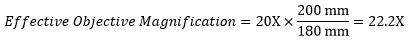 |
The effective magnification of the Olympus objective is 22.2X and the trinoculars have 10X eyepieces, so the image at the eyepieces has 22.2X × 10X = 222X magnification.
Sample Area When Imaged on a Camera
When imaging a sample with a camera, the dimensions of the sample area are determined by the dimensions of the camera sensor and the system magnification, as shown by Equation 2.
 |
(Eq. 2) |
The camera sensor dimensions can be obtained from the manufacturer, while the system magnification is the multiplicative product of the objective magnification and the camera tube magnification (see Example 1). If needed, the objective magnification can be adjusted as shown in Example 3.
As the magnification increases, the resolution improves, but the field of view also decreases. The dependence of the field of view on magnification is shown in the schematic to the right.
Example 4: Sample Area
The dimensions of the camera sensor in Thorlabs' previous-generation 1501M-USB Scientific Camera are 8.98 mm × 6.71 mm. If this camera is used with the Nikon objective and trinoculars from Example 1, which have a system magnification of 15X, then the image area is:
 |
Sample Area Examples
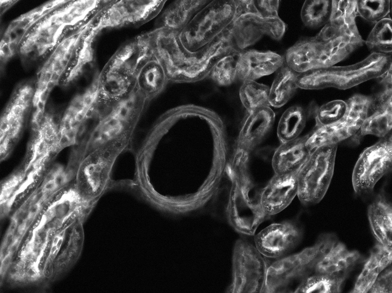
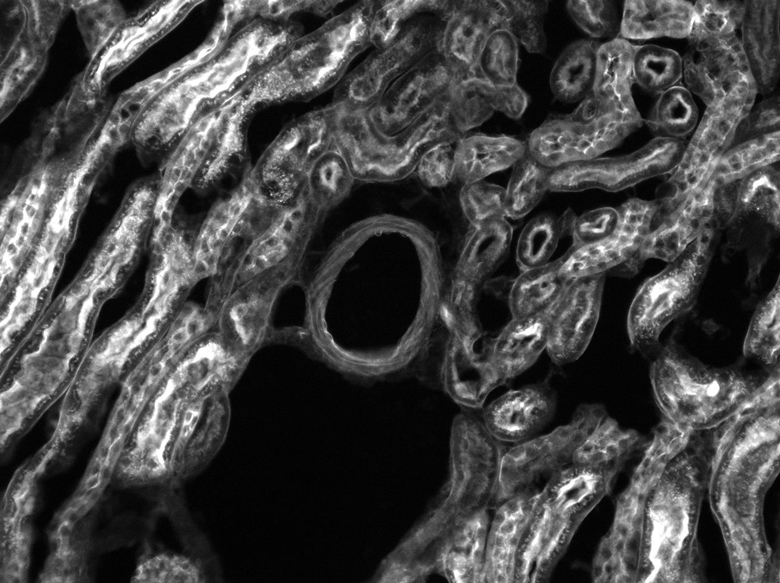
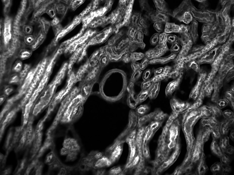
The images of a mouse kidney below were all acquired using the same objective and the same camera. However, the camera tubes used were different. Read from left to right, they demonstrate that decreasing the camera tube magnification enlarges the field of view at the expense of the size of the details in the image.
Resolution Tutorial
An important parameter in many imaging applications is the resolution of the objective. This tutorial describes the different conventions used to define an objective's resolution. Thorlabs provides the theoretical Rayleigh resolution for all of the imaging objectives offered on our site; the other conventions are presented for informational purposes.
Resolution
The resolution of an objective refers to its ability to distinguish closely-spaced features of an object. This is often theoretically quantified by considering an object that consists of two point sources and asking at what minimum separation can these two point sources be resolved. When a point source is imaged, rather than appearing as a singular bright point, it will appear as a broadened intensity profile due to the effects of diffraction. This profile, known as an Airy disk, consists of an intense central peak with surrounding rings of much lesser intensity. The image produced by two point sources in proximity to one another will therefore consist of two overlapping Airy disk profiles, and the resolution of the objective is therefore determined by the minimum spacing at which the two profiles can be uniquely identified. There is no fundamental criterion for establishing what exactly it means for the two profiles to be resolved and, as such, there are a few criteria that are observed in practice. In microscopic imaging applications, the two most commonly used criteria are the Rayleigh and Abbe criteria. A third criterion, more common in astronomical applications, is the Sparrow criterion.
Rayleigh Criterion
The Rayleigh criterion states that two overlapping Airy disk profiles are resolved when the first intensity minimum of one profile coincides with the intensity maximum of the other profile [1]. It can be shown that the first intensity minimum occurs at a radius of 1.22λf/D from the central maximum, where λ is the wavelength of the light, f is the focal length of the objective, and D is the entrance pupil diameter. Thus, in terms of the numerical aperture (NA = 0.5*D/f), the Rayleigh resolution is:
rR = 0.61λ/NA
An idealized image of two Airy disks separated by a distance equal to the Rayleigh resolution is shown in the figure to the left below; the illumination source has been assumed to be incoherent. A corresponding horizontal line cut across the intensity maxima is plotted to the right. The vertical dashed lines in the intensity profile show that the maximum of each individual Airy disk overlaps with the neighboring minimum. Between the two maxima, there is a local minimum which appears in the image as a gray region between the two white peaks.
 Click to Enlarge
Left: Two point sources are considered resolved when separated by the Rayleigh resolution. The gray region between the two white peaks is clearly visible.
Above: The vertical dashed lines show how the maximum of each intensity profile overlaps with the first minimum of the other.

Thorlabs provides the theoretical Rayleigh resolution for all of the imaging objectives offered on our site in their individual product presentations.
Abbe Criterion
The Abbe theory describes image formation as a double process of diffraction [2]. Within this framework, if two features separated by a distance d are to be resolved, at a minimum both the zeroth and first orders of diffraction must be able to pass through the objective's aperture. Since the first order of diffraction appears at the angle: sin(θ1) = λ/d, the minimum object separation, or equivalently the resolution of the objective, is given by d = λ/n*sin(α), where α is the angular semi-aperture of the objective and a factor of n has been inserted to account for the refractive index of the imaging medium. This result overestimates the actual limit by a factor of 2 because both first orders of diffraction are assumed to be accepted by the objective, when in fact only one of the first orders must pass through along with the zeroth order. Dividing the above result by a factor of 2 and using the definition of the numerical aperture (NA = n*sin(α)) gives the famous Abbe resolution limit:
rA = 0.5λ/NA
In the image below, two Airy disks are shown separated by the Abbe resolution limit. Compared to the Rayleigh limit, the decrease in intensity at the origin is much harder to discern. The horizontal line cut to the right shows that the intensity decreases by only ≈2%.
 Click to Enlarge
Left: Two point sources separated by the Abbe resolution limit. Though observable, the contrast between the maxima and central minimum is much weaker compared to the Rayleigh limit.
Above: The line cut shows the small intensity dip between the two maxima.

Sparrow Criterion
For point source separations corresponding to the Rayleigh and Abbe resolution criteria, the combined intensity profile has a local minimum located at the origin between the two maxima. In a sense, this feature is what allows the two point sources to be resolved. That is to say, if the sources' separation is further decreased beyond the Abbe resolution limit, the two individual maxima will merge into one central maximum and resolving the two individual contributions will no longer be possible. The Sparrow criterion posits that the resolution limit is reached when the crossover from a central minimum to a central maximum occurs.
At the Sparrow resolution limit, the center of the combined intensity profile is flat, which implies that the derivative with respect to position is zero at the origin. However, this first derivative at the origin is always zero, given that it is either a local minimum or maximum of the combined intensity profile (strictly speaking, this is only the case if the sources have equal intensities). Consider then, that because the Sparrow resolution limit occurs when the origin's intensity changes from a local minimum to a maximum, that the second derivative must be changing sign from positive to negative. The Sparrow criterion is thus a condition that is imposed upon the second derivative, namely that the resolution limit occurs when the second derivative is zero [3]. Applying this condition to the combined intensity profile of two Airy disks leads to the Sparrow resolution:
rS = 0.47λ/NA
The image to the left below shows two Airy disks separated by the Sparrow resolution limit. As described above, the intensity is constant in the region between the two peaks and there is no intensity dip at the origin. In the line cut to the right, the constant intensity near the origin is confirmed.
 Click to Enlarge
Left: Two Airy disk profiles separated by the Sparrow resolution limit. Note that, unlike the Rayleigh or Abbe limits, there is no decrease in intensity at the origin.
Above: At the Sparrow resolution limit, the combined intensity is a constant near the origin. The scale here has been normalized to 1.

References
[1] Eugene Hecht, "Optics," 4th Ed., Addison-Wesley (2002)
[2] S.G. Lipson, H. Lipson, and D.S. Tannhauser, "Optical Physics," 3rd Ed., Cambridge University Press (1995)
[3] C.M. Sparrow, "On Spectroscopic Resolving Power," Astrophys. J. 44, 76-87 (1916)
Click to Enlarge
Old Objective Packaging

Click to Enlarge
New Objective Packaging
Smart Pack Goals
- Reduce Weight of Packaging
- Increase Usage of Recyclable Materials
- Improve Packing Integrity
- Decrease Shipping Costs
Thorlabs' Smart Pack Initiative is aimed at minimizing waste while providing adequate protection for our products. By eliminating any unnecessary packaging, implementing design changes, and utilizing eco-friendly materials, this initiative seeks to reduce the environmental impact of our product packaging.
The new super achromatic microscope objective packaging is made from over 60% recycled paper products and weighs 25.44 g less than the old packaging. The transition from foam and non-recycled cardboard to recycled paper products results in a 68.05% reduction in the amount of CO2 produced per kg of packing materials. All products on this page have transitioned, or are in the process of transitioning to recycled paper.
As we move through our product line, we will indicate re-engineered, eco-friendly packaging with our Smart Pack logo, which can be seen in the image to the right.
| Posted Comments: | |
Biao SUN
(posted 2024-11-05 10:11:42.883) Since the Objective is designed for 2P system,you may provide the dispersion of the objective across the transmission band, at least 700-1300nm cdolbashian
(posted 2024-11-13 03:23:01.0) Thank you for reaching out to us with this inquiry. I have contacted you directly to share these data with you. user
(posted 2024-07-04 12:22:40.993) Would any of these objectives be cryo-compatible? cdolbashian
(posted 2024-07-19 02:58:35.0) Thank you for reaching out to us with this inquiry. We discussed your application, and the fact that you need to use these objectives in a 4 Kelvin environment. Unfortunately, as these were not designed for this environment, it is unlikely that you could use one of these scopes to the specced performance. I have contacted you directly to discuss possible alternatives. Hannes Kamin
(posted 2024-06-19 13:51:17.263) Hi Thorlabs Team,
can the TL10X-2P be used with cleared samples? I want to dipp in into clearing media with high refractive index. Is the objective resistant to ECI or BABB (Ethyl cinnamate or Benzyl / Alcohol / Benyl Benzoat) when dipping into that media?
Thank you very much cdolbashian
(posted 2024-06-28 11:32:27.0) Thank you for reaching out to us with these inquiries. This objective can indeed be used with cleared samples. When considering dipping media, we would advise only non corrosive immersion oils or water. KYLE LILLIS
(posted 2024-02-09 15:35:00.233) We recently purchased the TL10X-2P for in vivo imaging. Can you tell me how you recommend sterilizing this objective? I assume it can't be autoclaved? How about EtO? cdolbashian
(posted 2024-02-19 10:51:55.0) Thank you for reaching out to us with this usage inquiry. We would not recommend autoclaving this component. We would recommend regular, normal cleaning immediately after each use, The lens paper should be immersed in an appropriate solvent to remove any oils used and you should clean the lens without endangering it. We advise using blended alcohol, anhydrous alcohol, or a lens-cleaning solution. Xindong Song
(posted 2021-02-25 16:31:18.73) Hi Thorlabs, we are very interested in getting the TL10X-2P objective for in vivo 2p imaging. But before we place the order, we wonder if we can talk to any other customers about their experience with the objective. Thank you. YLohia
(posted 2021-03-05 10:00:19.0) Hello, thank you for contacting Thorlabs. Unfortunately, we cannot share customer information due to privacy concerns. That being said, you can look through publicly available literature for mentions of this lens and contact the authors of those papers. For example, here is a Google Scholar search with a few relevant results: https://scholar.google.com/scholar?hl=en&as_sdt=0%2C31&q=TL10X-2P&btnG= Michael Orger
(posted 2020-11-06 06:51:53.37) Hi, Can you define Forward and Reverse for the TL10X-2P zemax black box files? It seems to be the opposite of what I expect, but I am not sure if it is a misunderstanding on my part. Thanks! asundararaj
(posted 2020-11-10 09:40:01.0) Thank you for contacting Thorlabs. Forward is typically defined as sending a collimated light into the objective, and the reverse is defined as sample being on the object side. Forward is always from collimation to focus. Gabriel Martins
(posted 2019-07-17 06:54:01.707) good morning,
do you have information on how the 10x performs with cleared samples, ie, samples in medium with refractive index of ~1.52?
Would it be possible to test the objective with our samples?
Thanks in advance,
Gaby asundararaj
(posted 2019-07-23 10:08:15.0) Thank you for contacting Thorlabs. Yes, the TL10X-2P objective can be used with cleared samples. You would need to set the spherical collar to the appropriate setting. You can find a procedure for calculating the correct setting in the Correction Collar tab of this page. I have contacted you directly about being able to offer a loan unit. Denis Pristinski
(posted 2019-07-12 12:53:38.397) Is Zemax black box model coming for TL10X-2P? YLohia
(posted 2019-07-16 09:02:38.0) Hello, thank you for contacting Thorlabs. The Zemax model for this can be found here : https://www.thorlabs.com/_sd.cfm?fileName=TTN142896-S02.zar&partNumber=TL10X-2P a.scagliola2
(posted 2018-11-05 12:38:56.0) Do you have a model of the objective with the principal planes? nbayconich
(posted 2019-03-04 01:17:21.0) Thank you for contacting Thorlabs. The principal plane will be located approximately 16mm in front of the objective lens or 16mm after the m25 x0.75 threading. I will reach out to you directly with more information. a.andreski
(posted 2017-11-28 15:40:24.44) Do these objectives have a flat field of view (are they plan)?
If I use the TL2X-SAP with a TTL100A tubelens, what is the maximum object field of view that is possible without abberations?
Thanks. tfrisch
(posted 2017-12-15 04:35:36.0) Hello, thank you for contacting Thorlabs. The Field of View will be flat, yes. TL2X-SAP will be diffraction limited over its full Field of View. I will reach out to you directly with details on the Strehl ratio. ludoangot
(posted 2016-11-07 15:31:29.6) Which tube lens do you recommend to match the extended transmission of these microscope lenses in the deep blue / UV (your recent TTL200 is for 400 to 700nm)? tfrisch
(posted 2016-11-10 10:24:31.0) Hello, thank you for contacting Thorlabs. I would typically recommend TTL200 which performs well over the range of TL2X-SAP and TL4X-SAP. You can see some performance graphs here: https://www.thorlabs.us/newgrouppage9.cfm?objectgroup_id=5834&tabname=Graphs |

 Zoom
Zoom
Click to Enlarge
Click Here for Full-Size Image
10 kΩ resistor and diode surface mounted to a circuit board, imaged using the TL1X-SAP objective with reflected illumination from a FRI61F50 Ring Light and a color camera. The objective's telecentric design provides constant magnification through the depth of the image.
- Ideal for Machine Vision Applications
- Telecentric Design with Wave Plate for Reducing Back Reflections
- M25 x 0.75 Threading
Click for Details
The TL1X-SAP objective includes a removable wave plate that is attached to end of the objective barrel with magnets.
The TL1X-SAP Super Apochromatic Objective provides diffraction-limited axial color performance over 440 nm to 700 nm. The telecentric design provides constant magnification regardless of the object's distance or location in the field of view; see the Telecentric Tutorial tab for more information. This objective has a Ø22 mm field of view and is ideal for machine vision applications. It includes a removable waveplate that minimizes back reflections when used with an epi-illuminated system, thus enabling an increase in contrast. Magnets in the objective housing secure the wave plate in place. White markings on the 1X objective barrel and a black dot on the wave plate provide a reference when rotating the wave plate.
The full-size download of the circuit board image to the right should be viewed using ThorCam, ImageJ, or other scientific imaging software. It may not be displayed correctly in general-purpose image viewers.
| Key Specifications | ||||||||||||||
|---|---|---|---|---|---|---|---|---|---|---|---|---|---|---|
| Item # | AR Coating Wavelength Range |
Mag. | Numerical Aperture |
Working Distance |
Parfocal Length |
Cover Glass Thickness |
Threading | Recommended Microscopy Techniques | ||||||
| Confocal | Two-Photon | Brightfield | Darkfield | Dodt | DIC | Fluorescence | ||||||||
| TL1X-SAP | 420 - 700 nm | 1X | 0.03 | 8.0 mma | 95.0 mma | 0 - 0.5 mm | M25 x 0.75 | - | ||||||

 Zoom
Zoom- High Numerical Aperture for Low-Light and Widefield Imaging
- M25 x 0.75 Threading
These general-purpose objectives provide diffraction-limited axial color performance over 400 nm to 750 nm. They offer high-quality performance when used with a variety of imaging modalities and are useful for viewing large regions of a sample. The TL2X-SAP objective features a large Ø11 mm field of view while still retaining fine details over the whole field (Figures 1 and 2 below). The 4X magnification of the TLX4X-SAP can resolve finer details than its 2X counterpart, while the Ø5.5 mm field of view still provides a sense of scope and place within the sample (Figures 3 and 4 below). The long working distance of each objective provides ample room for micromanipulators.
The full-size downloads of Figures 1, 3, and 4 should be viewed using ThorCam, ImageJ, or other scientific imaging software. They may not be displayed correctly in general-purpose image viewers.
 Click to Enlarge
Click Here for Full-Size Image
Figure 1: Embryonic zebrafish embryo imaged using the TL2X-SAP objective, white light illumination, and a color camera. The image captures the full length of the zebrafish while still retaining fine details.
 Click for Details
Click Here for Full-Size Image
Figure 2: Sunstone imaged using the TL2X-SAP objective. This image captures a large section of sunstone while retaining excellent resolution across the field. Image courtesy of Stephen Challener.
 Click to Enlarge
Click Here for Full-Size Image
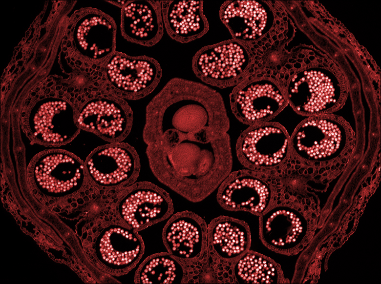
Figure 3: Dicot flower bud imaged using the TL4X-SAP objective and monochrome camera in a DIC setup.
 Click to Enlarge
Click Here for Full-Size Image
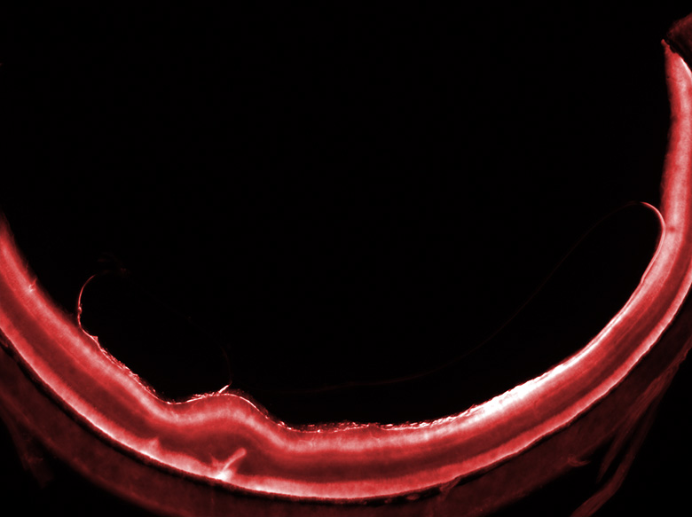
Figure 4: Confocal fluorescence image of a mouse retina labeled with GFP, taken using the TL4X-SAP objective.
| Key Specifications | ||||||||||||||
|---|---|---|---|---|---|---|---|---|---|---|---|---|---|---|
| Item # | AR Coating Wavelength Range |
Mag. | Numerical Aperture |
Working Distance |
Parfocal Length |
Cover Glass Thickness |
Threading | Recommended Microscopy Techniques | ||||||
| Confocal | Two-Photon | Brightfield | Darkfield | Dodt | DIC | Fluorescence | ||||||||
| TL2X-SAP | 350 - 700 nm | 2X | 0.10 | 56.3 mm | 95.0 mm | 0 - 0.5 mm | M25 x 0.75 | - | ||||||
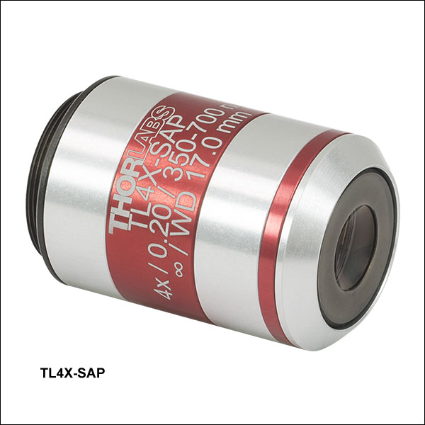
| TL4X-SAP | 350 - 700 nm | 4X | 0.20 | 17.0 mm | 60.0 mm | 0 - 0.5 mm | M25 x 0.75 | - | ||||||

 Zoom
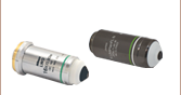
ZoomTL10X-2P Super Apochromatic Microscope Objective
- Dry Objectives Ideal for Two-Photon Microscopy
- Correction Collar Enables Use with Samples in a Variety of Media
- M32 x 0.75 Threading
The TL10X-2P Super Apochromatic and TL15X-2P Plan Apochromatic Improved Visible (APO VIS+) Objectives combine the diffraction limited axial color performance at visible wavelengths of our other objectives with excellent transmission out to 1300 nm, making these objectives ideal for multiphoton imaging applications (see the Graphs tab for details). For more information about how these objective classes are defined, see the Objective Tutorial tab. The 10X objective combines a 0.50 NA with a long 7.77 mm working distance, providing ample space for equipment to manipulate the sample. The 15X objective features a high 0.70 NA for collecting two-photon fluorescence signals and a working distance of 2.6 mm. A correction collar on each objective allows adjustment for spherical aberrations introduced by imaging through aqueous solutions or thick cover glasses, without the need for water dipping or oil immersion (see the Correction Collar tab). The TL15X-2P objective additionally features a locking mechanism to fix the correction collar in place for improved repeatability.
 Click to Enlarge
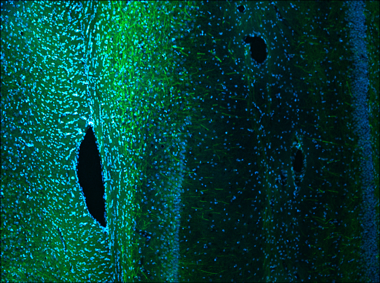
Click Here for Full-Size Image
Wild Type Mouse Brain Section (30 µm) Tagged with DAPI (405 nm) and Alexa 488 Anti-Neurofilament Taken with TL10X-2P Objective (Courtesy of Lynne Holtzclaw of the National Institutes of Health)
Note that for best performance, the front focal plane of your system's tube lens should be placed at the objective's aperture stop. For most objectives, this stop coincides with the back element at the shoulder. The aperture stops in Item #s TL10X-2P and TL15X-2P are located 42.0 mm and 52.2 mm from their shoulders, respectively. Without filling this stop, vignetting may occur. For example, Thorlabs' TTL200MP tube lens' focal plane is located at 228 mm from the shoulder of the tube lens. Therefore, the physical separation between the front element of the tube lens and the shoulders of the TL10X-2P and TL15X-2P objectives should be 186 mm and 175.8 mm, respectively. These examples are illustrated in the alignment diagrams that can be viewed by clicking on the blue info icons (![]() ) in the table below.
) in the table below.
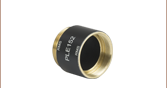
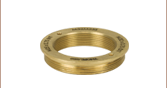
Due to the large outer diameter of this objective's housing, it may not mate properly with nosepieces that have recessed M32 x 0.75 internal threads such as Item #s CSN200 and CSN210. In this case, the M32M32S brass microscope adapter has external and internal M32 x 0.75 threads that can provide additional clearance between the edge of the objective housing and the mount.
The full-size download of the mouse brain image to the lower right should be viewed using ThorCam, ImageJ, or other scientific imaging software. It may not be displayed correctly in general-purpose image viewers.
| Key Specifications | |||||||||||||||
|---|---|---|---|---|---|---|---|---|---|---|---|---|---|---|---|
| Item # | AR Coating Wavelength Range |
Mag. | Numerical Aperture |
Working Distance |
Parfocal Length |
Cover Glass Thickness |
Threading | Alignment Diagram |
|||||||
| TL10X-2P | 400 - 1300 nm | 10X | 0.50 | 7.77 mm | 95.0 mm | 0 - 2.6 mm | M32 x 0.75 |  |
|||||||
| TL15X-2P | 15X | 0.70 | 2.6 mma | 75.0 mm | 0 - 2.8 mm |  |
|||||||||
| Recommended Microscopy Techniques | ||||||
|---|---|---|---|---|---|---|
| Confocal | Two-Photon | Brightfield | Darkfield | Dodt | DIC | Fluorescence |
| - | ||||||